
Phase diagrams
Phase diagrams is part of a free web series, GWB Online Academy, by Aqueous Solutions LLC.
What you need:
- GWB Professional recommended
-
Input files:
 CuSH2O.ph2, O2Solubility.ph2, AlSolubility.ph2
Download this unit to use in your courses:
- Lesson plan (.pdf)
- PowerPoint slides (.pptx)
Click on a file or right-click and select “Save link as…” to download.
Introduction
Phase2 is a program for calculating phase and predominance diagrams of virtually any type. The program works by tracing a series of stacked reaction paths across the diagram.

Each traverse is conceptually identical to a React simulation. As such, Phase2 can account not only for multicomponent chemical equilibrium, but reaction kinetics, external buffers, sorption and surface complexation, stable isotope fractionation, and, in fact, any of React's many capabilities.
A Phase2 diagram differs from a simple diagram of the type constructed by Act2 and Tact in that each point in the diagram represents the complete solution to the equations describing the system's distribution of mass. If you were to use Phase2 to calculate an Eh-pH diagram, for example, you would find that, unlike the result from Act2, the boundary lines are curved, rather than linear. Because of the calculation's completeness, some Phase2 diagrams differ qualitatively from their Act2 counterparts. For this reason, the diagrams are sometimes referred to as “true” Eh-pH or “true” activity diagrams.
Task 1: Speciation diagram
As a first example, we construct a “true” fO2-pH diagram for the copper-sulfur-water system at 250°C. Double-click on file “CuSH2O.ph2” to launch Phase2 and move to the Basis pane
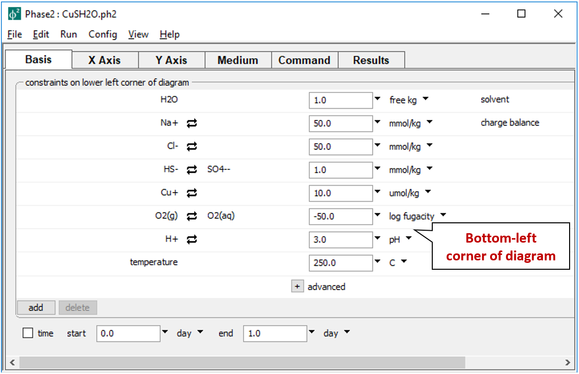
Here we constrain the chemical system at the bottom-left corner of the diagram: the background electrolyte is 50 mmol/kg NaCl, and the fluid contains 1 mmol/kg sulfur and 10 µmol/kg copper. The corner marks a log fugacity of −50 and a pH of 3.
The Y Axis pane sets up the staging axis
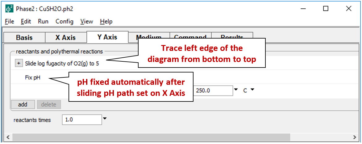
such that the logarithm of oxygen fugacity slides to 5, while pH holds constant.
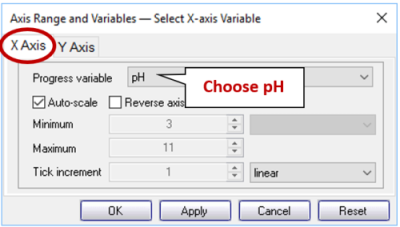
In contrast, the X Axis pane
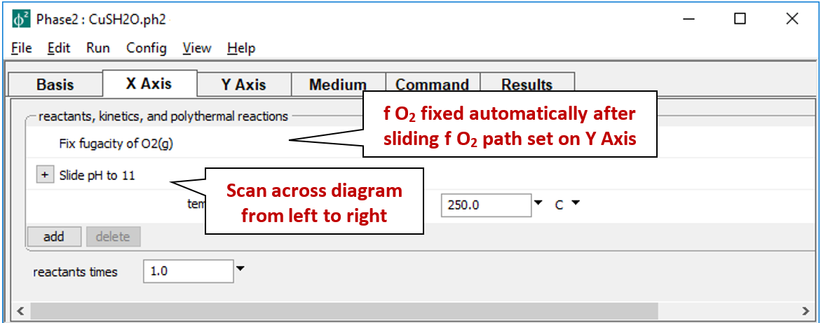
fixes fugacity, but slides pH to 11.
On Config → Output…, note the grid resolution
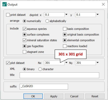
Computing time and memory use increases as the product of the x- and y-direction resolutions, so you should avoid setting overly large values.
While in the Output dialog, set a suffix “_CuSH2O”, then click OK.
Move to the Results pane and click  to trigger the calculation. When the program finishes, choose
  to open dataset “Phase2_plot_CuSH2O.p2p”, which holds the calculation results, in program P2plot.
In P2plot select Plot → 2D Diagram. When the diagram displays, double-click on one of the axis variables (or go to Format → Axis Range and Variables…) and on the X Axis tab set “Progress Variable” to “pH”.
then, on the Y Axis tab, set the variable for the y axis to “log f O2(g)”.
Next, click on Format → Predominance Map… to expose the Predominance Map dialog. Check the box next to “Predominance Map”, if it is not already, and next to “Variable to map”, choose “Cu+”
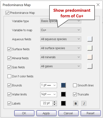
Click on Apply.
What are the predominant copper-bearing species and minerals at 250°C as a function of pH and oxidation state? What are the predominant sulfur-bearing species?
From the calculation results, we can plot predominance for Cu+
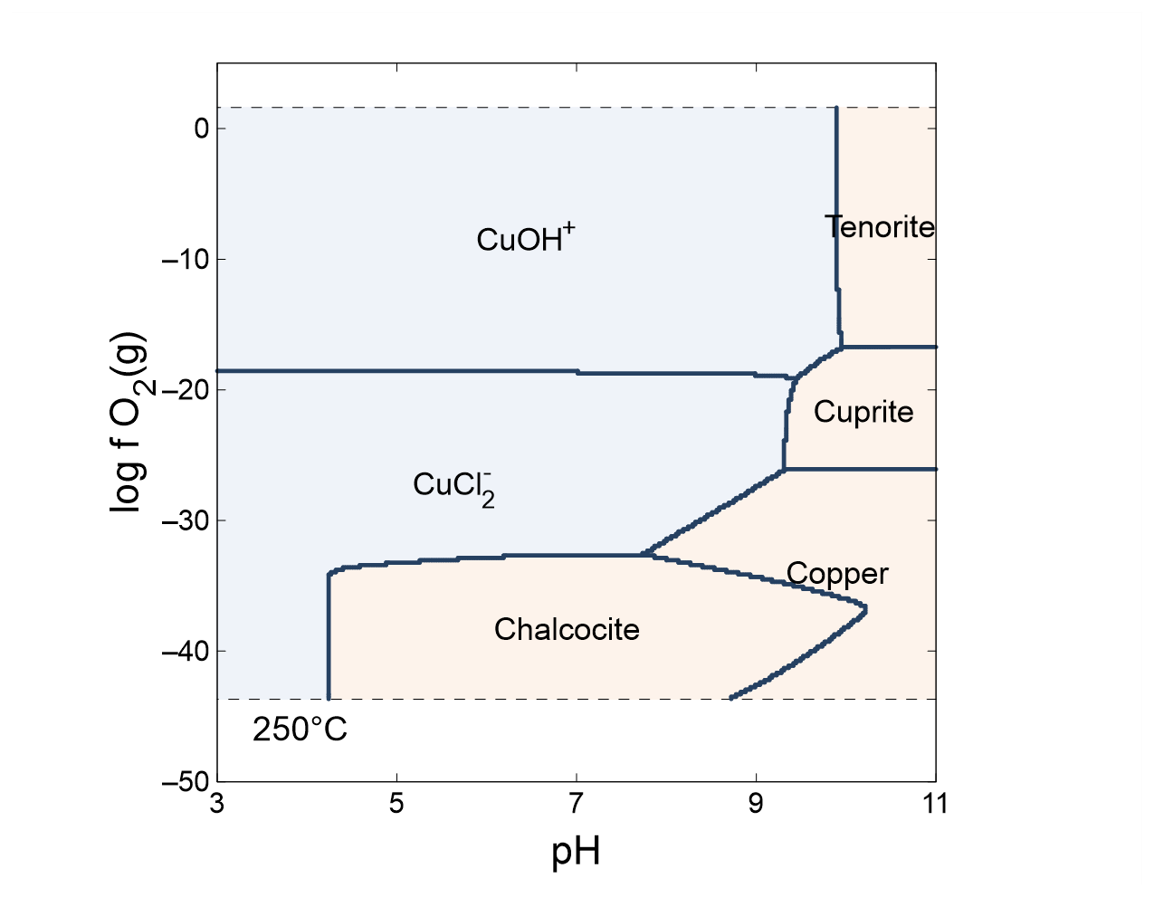
Under reducing conditions and neutral pH, the iron-sulfide mineral chalcocite predominates, wherease elemental copper predominates at higher pH. At somewhat higher oxidation states, first the cuprous mineral cuprite and then the cupric mineral tenorite predominate. Note that a mineral's field of stability may be somewhat larger than its area of predominance.
Note the curvature of the bounding lines, as opposed to equilibrium lines in Act2, which are always straight.
By changing the “Variable to map” pulldown to “SO4--”, we can display predominance of the sulfate component
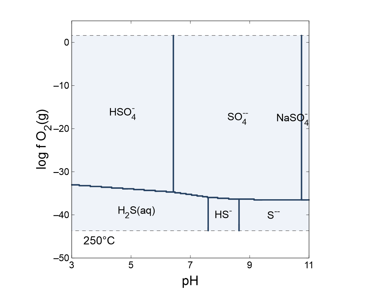
No minerals predominate under these conditions. Sulfide species predominate at low fO2, but sulfate species predominate at higher oxidation states.
The plot is truncated at low and high fO2 by the upper and lower stability limits of water. To extend the diagram, return to the Predominance Map dialog, uncheck “Truncate”, and click on Apply.
P2plot can diagram cross-sections through any diagram. You can make x-y plots of a broad range of variables such as pH, species concentration, mineral mass, gas pressure, isotopic composition, and so on.
To plot along a cross-section, select Plot → Cross section Plot…. On the X Axis pane, set “Orientation” to “Along scanning paths” and choose to plot “pH” among the “Chemical parameters”; under Y Axis, set “Variable type” to “Species concentration”, “Filter” to “SO4--”, “Display” to “Several values at one step along y”, and then set a “linear” scale. Click on Select all, if necessary. Moving to the Step pane, set “Progress variable” to “log f O2(g)” and pick a value. The bottom edge of the 2D diagram, which corresponds to a log fugacity of −50, is listed first. How does speciation change as you move from the bottom to the top of the diagram?
The cross-section plot reveals details of the 2D rendering
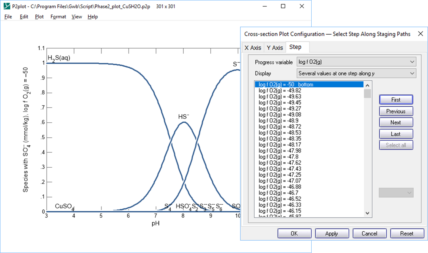
As shown in the 2D predominance area diagram, sulfide species give way to sulfate species at higher oxidation states.
Task 2: Gas solubility
In this example we diagram the solubility in water of atmospheric O2(g) as a function of salinity and temperature. Our strategy is to define a dilute fluid in equilibrium with the atmosphere at 0°C to occupy the lower-left corner of the diagram. We will then set temperature to increase along the staging axis, and salinity along the scanning axis, while holding O2(g) fugacity constant across both axes.
Begin by double-clicking on file “O2Solubility.ph2” to launch Phase2. The Basis pane
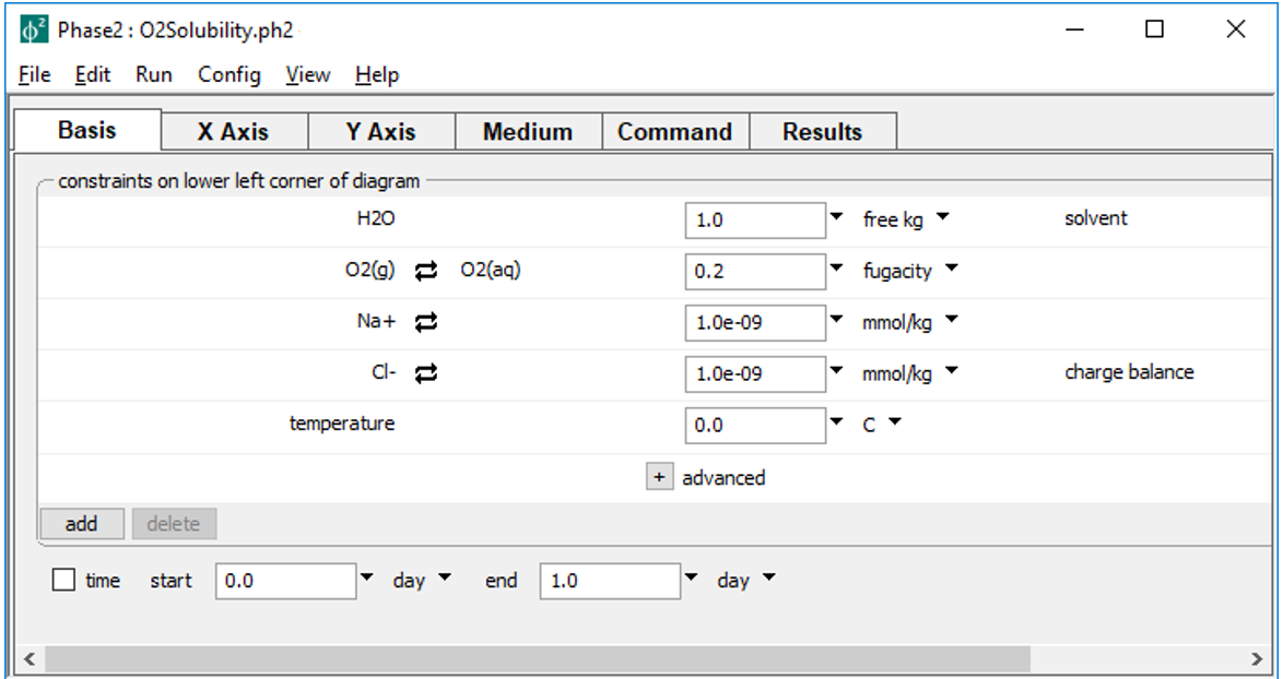
sets the bottom left corner of the diagram, whereas the Y Axis pane
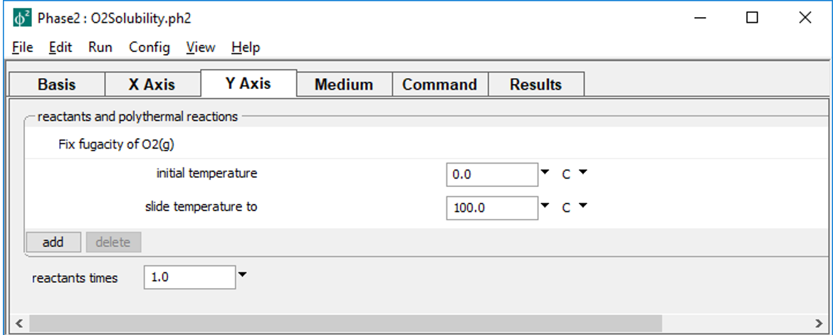
slides temperature along the staging path, and the X Axis pane
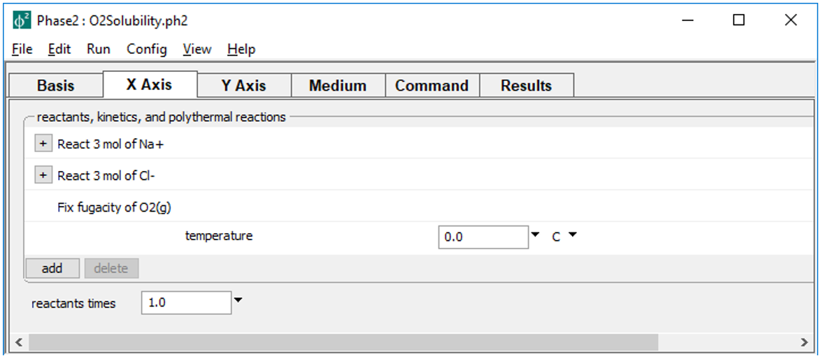
sets up a titration of 3 mol of Na+ and Cl- as simple reactants along the scanning paths.
The simulation, then, consists of a series of isothermal titration paths, each traced at fixed oxygen fugacity, and each maintaining the temperature of its point of departure from the staging path.
On Config → Output…, set a suffix “_O2Solubility”
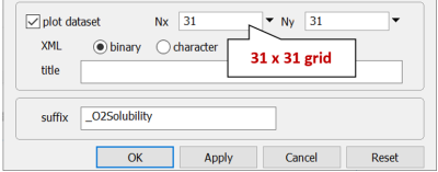
While there, you can coarsen the grid to calculate and render results more rapidly. Decrease Nx and Ny from “301” to “31”. Later, you can set a finer grid and rerun the calculation. Click OK.
Press the button on the Results pane to trace the calculation.
Press to launch P2plot, then select Plot → 2D Diagram. Double-click on one of the axis variables (or go to Format → Axis Range and Variables…), then set the x axis progress variable to “Cl- in system”, with units of “mmol/kg”, and the y axis variable to “Temperature”. Now, select Format → Contour… to expose the contour plot dialog. Choose “Species concentration”, “All species”, “O2(aq)”, “mmol/kg”, and “Linear” in the top five fields, then check the box next to “Contour Lines” and click on Apply. Under Format → Color Map…, choose the same settings and hit Apply.
If you set a coarse grid earlier, you can return to Phase2 and set Nx and Ny to “301”, then rerun the calculation. Your plot will update automatically.
How does oxygen solubility vary across the conditions of the diagram?
Oxygen solubility decreases with increased temperature and salinity.
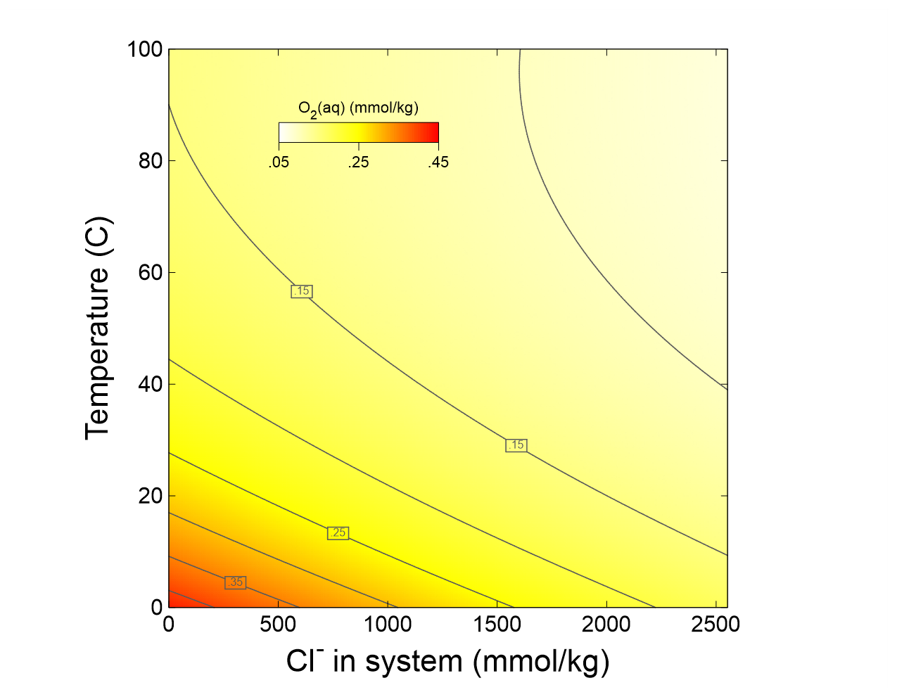
The diagram reflects how the log K of the reaction between O2(g) and O2(aq) decreases with temperature, while the activity coefficient of O2(aq) increases with ionic strength. The latter effect is commonly known as the “salting out” effect.
Task 3: Mineral solubility
The input file “AlSolubility.ph2” calculates the solubility of aluminum in the presence of quartz as a function of pH and the system's aluminum content. Double-click the file to launch Phase2. The Basis pane
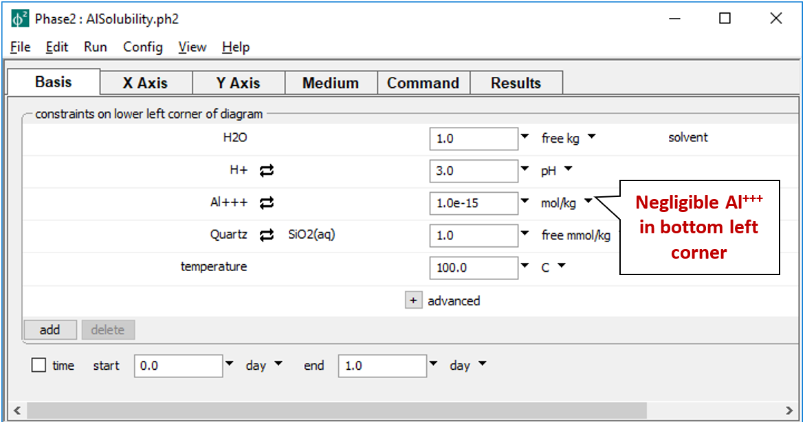
describes the starting point for our calculation, a pH 3 fluid in equilibrium with quartz at 100°C. The fluid carries a near-zero mass of dissolved aluminum. We don't include a background electrolyte, so charge balancing is disabled.
The Y Axis pane
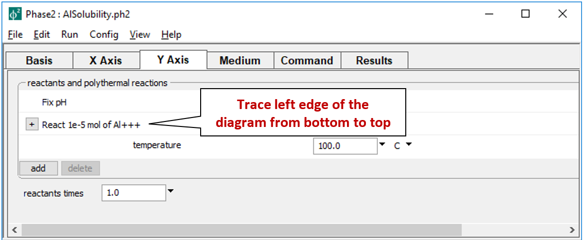
shows the staging path, along which 10 µmol of Al+++ is titrated into to the system, while pH is held constant.
On the X Axis pane
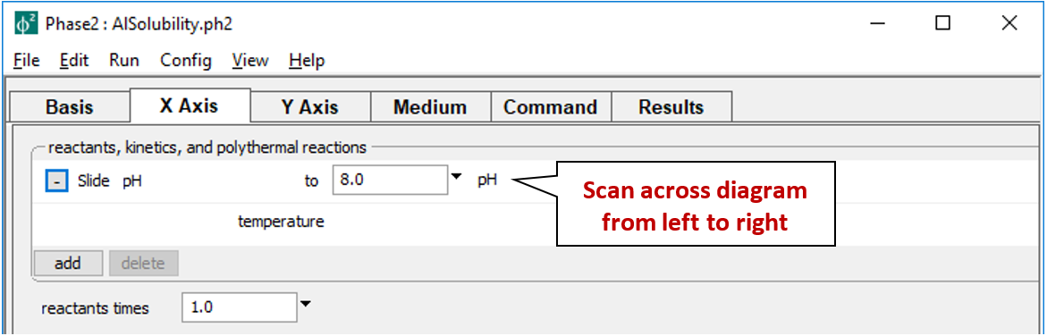
pH is set to slide from 3, the starting point, to a final value of 8.
On the Config → Stepping… dialog
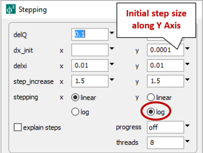
we set logarithmic stepping along the y axis, with an initial step size of 10−4. Since we're ultimately adding 10−5 moles of Al+++, Phase2 will add 10−4×10−5 = 10−9 moles to the initially negligible mass on the first step, then exponentially larger aliquots as it takes subsequent steps.
On Config → Output…, set a suffix “_AlSolubility”. As before, you may wish to make an initial calculating using a course grid. Later, once the plot appearance is to your liking, you can rerun the calculation and the open plot will update automatically.
Press the button on the Results pane to trace the calculation. Start P2plot by clicking on the and select Plot → 2D Diagram. Double-click on the x axis label and set “Progress Variable” to “pH”. Move to the Y Axis tab and set “Progress Variable” here to “Al+++ in system” with a log scale. Adjust the tick increment on each axis, if you wish, by de-selecting “Auto-scale”, and click OK.
Next, select Format → Assemblage Map…, check the box at the top of the dialog, and click OK. Select Format → Contour Map… and check the box at the top of the dialog. Next to “Variable type”, choose “Components in fluid”, set “Variable to contour” to “Al+++”, and for “Variable units”, set “umol/kg”. Make sure “Type of plot” is “Log”, and adjust the point size and color of the contour lines to your liking, and click OK.
Under what conditions is kaolinite stable? Where is aluminum most soluble?
The mineral is most soluble at the low and high pH extremes of the diagram, and least soluble around pH 5.
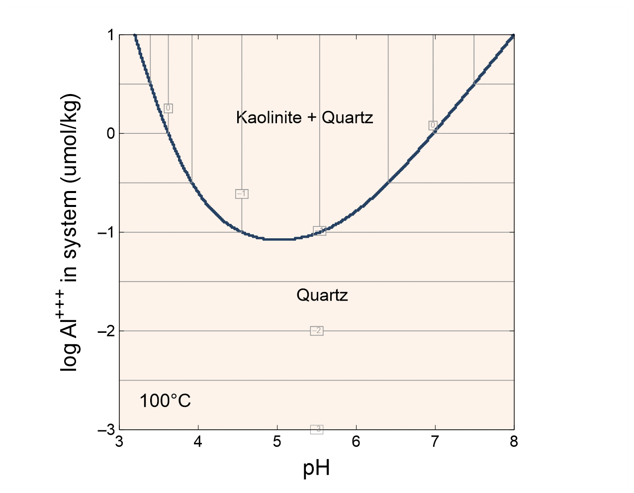
The blue bounding line represents the solubility of kaolinite as a function of pH, and contours represent the log of dissolved aluminum concentration. Everywhere below the curve, the fluid is undersaturated with respect to kaolinite; all of the aluminum in the system is in solution. Above the curve, kaolinite is stable—any aluminum in excess of the solubility precipitates, so the dissolved aluminum concentration depends only on pH.
Authors
Craig M. Bethke and Brian Farrell. © Copyright 2016–2025 Aqueous Solutions LLC. This lesson may be reproduced and modified freely to support any licensed use of The Geochemist's Workbench® software, provided that any derived materials acknowledge original authorship.
References
Bethke, C.M., 2022, Geochemical and Biogeochemical Reaction Modeling, 3rd ed. Cambridge University Press, New York, 520 pp.
Bethke, C.M., B. Farrell, and M. Sharifi, 2025, The Geochemist's Workbench®, Release 17: GWB Reaction Modeling Guide. Aqueous Solutions LLC, Champaign, IL, 219 pp.
Comfortable with phase diagrams?
Move on to the next topic, Mass Transport, or return to the GWB Online Academy home.