
Stability diagrams
Stability Diagrams is part of a free web series, GWB Online Academy, by Aqueous Solutions LLC.
What you need:
- GWB Essentials recommended
Download this unit to use in your courses:
- Lesson plan (.pdf)
- PowerPoint slides (.pptx)
Introduction
Act2 and Tact calculate stability diagrams on activity, fugacity, and temperature axes. They additionally calculate solubility diagrams and can be overlain with scatter data from GSS spreadsheets or traces of React runs.
The basis is the set of aqueous species, minerals, and gases with which we choose to
- Write chemical reactions
- Express composition
The number of basis entries is the number of components in the system, which is fixed by the laws of thermodynamics.
By convention, we will choose as the basis
- Water, the solvent
- Each mineral in equilibrium with the system
- Each gas at known fugacity or partial pressure
- Important aqueous species
In any GWB model, you follow a similar set of steps:
- SWAP. Prepare your calculation by swapping into the basis the species with which you wish to write reactions, including any coexisting minerals and gases. For an activity-activity diagram, the basis includes the main species and axis variables.
- SET. Set constraints on the system, perhaps including temperature, total concentration, species' activity, gas fugacity or partial pressure, etc.
- GO. Select Run → Go to let the program trace the reaction path, calculate and display the diagram, or balance the reaction.
- REVISE. Change the basis, add new components, or alter any of the specifications for your model. Then select Run → Go to render the new result.
Task 1 - Activity-activity diagrams
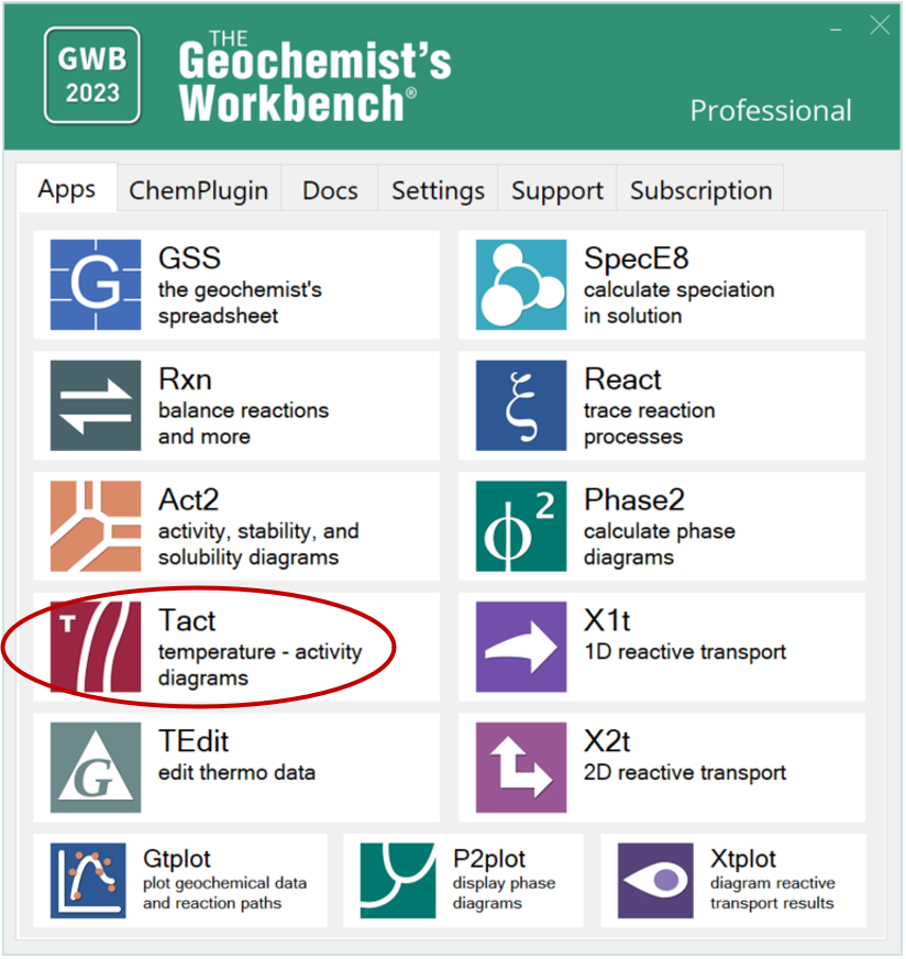
Act2 calculates stability diagrams in activity and fugacity coordinates. To calculate a redox-pH diagram for iron, for example, start Act2 from the GWB dashboard
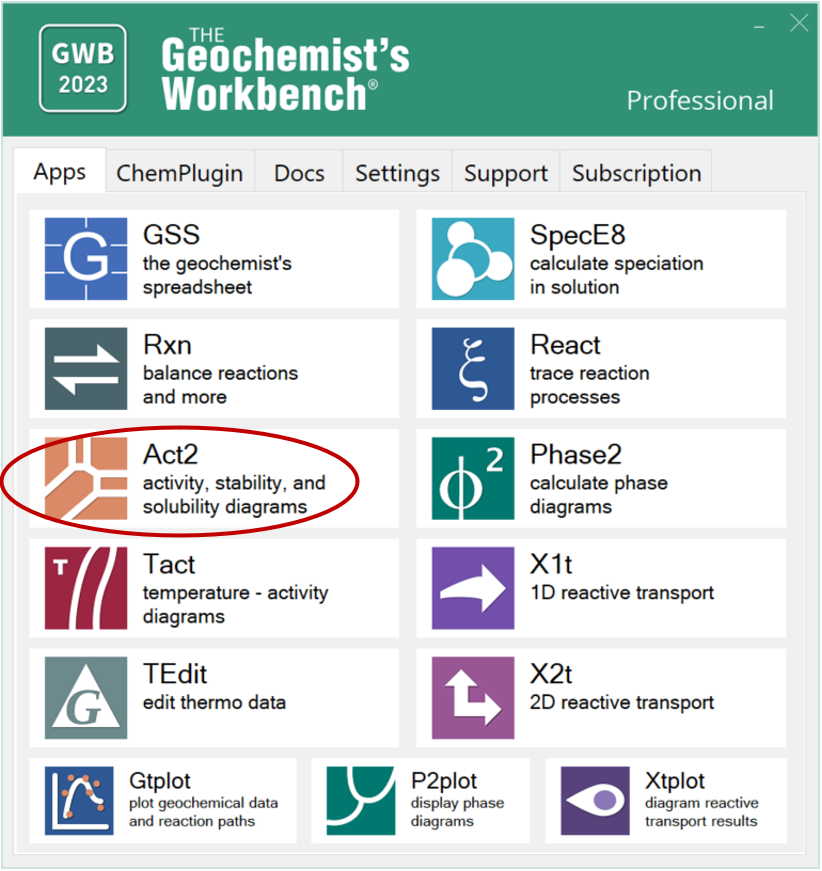
and move to the Basis pane:
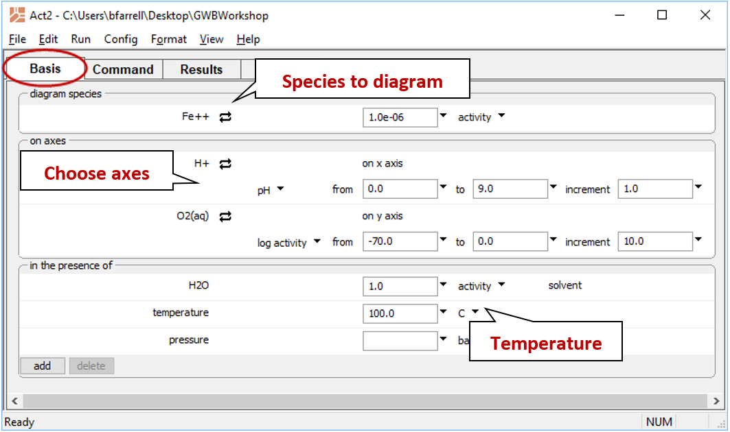
- Under “diagram species”, select “Fe++” and set activity to “10^-6”.
- Under “on axes”, select “H+” for x and set the unit to “pH”. Set the axis to range up to “9”.
- For y, choose “O2(aq)” set the axis to range from “−70.0” to “0”.
- Set “temperature” to 100°C.
The pane should look like
Move to the Plot pane to view your diagram.
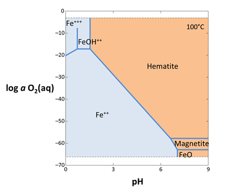
The dashed lines that limit the top and bottom of the plot show the stability limits of water at 1 atmosphere pressure. The diagram shows various aqueous species, minerals, and gases that are predominant under the chosen conditions. Each is formed from some combination of species in our basis set: Fe++, H+, O2(aq), and H2O.
Each solid line on the diagram represents a reaction between species at equilibrium. You can click on a line to see its stoichiometry in a tooltip. In Rxn, you can additionally find the equation for the equilibrium line, as described in the Equilibrium lines section of the Online Academy.
Return to the Basis pane and recalculate the diagram assuming Fe2+ activities of 10−4 and 10−8. (Note that CTRL+G in the GWB apps is a shortcut for Run → Go.) Comparing the three plots, do the positions of the reaction lines between aqueous species change? The reaction lines between minerals?
We've overlain the results from three separate diagrams into one plot using MS PowerPoint
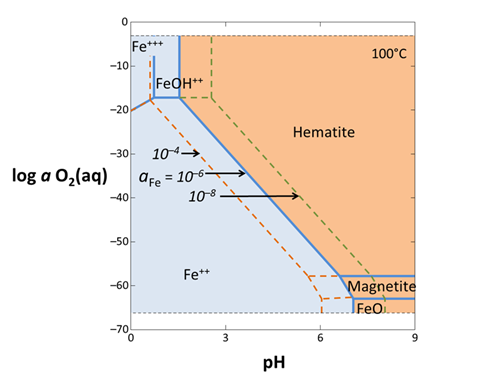
As you can see, the reaction lines between a mineral and aqueous species, such as between Hematite and Fe++, shift depending on the activity set for Fe++. Reactions lines between pairs of species do not shift as you change activity, nor do reaction lines between pairs of minerals.
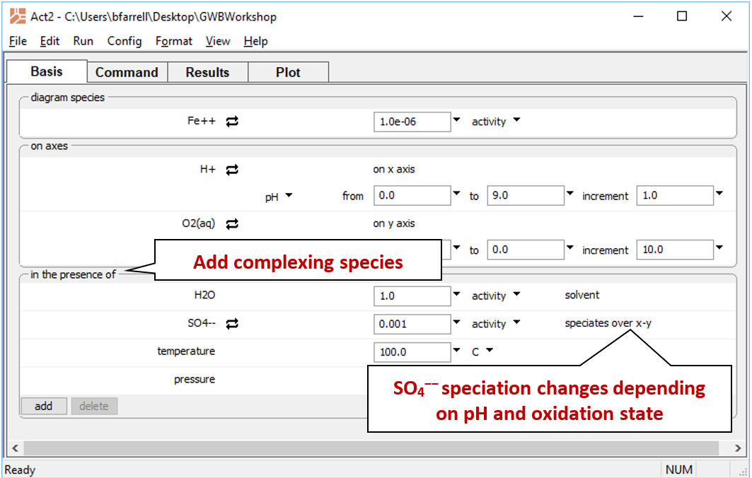
You can add complexing species to the diagram on the Basis pane, under “in the presence of”. Some complexing species react across the diagram coordinates. For example, SO42− reacts under changing Eh or pH to form HSO4−, HS−, H2S(aq), and so on. To correctly include SO42− as a complexing species, we need to calculate a mosaic diagram.
Revert the Fe2+ activity to “10^-6”. Under “in the presence of”, click on add and select “SO4--”. Set the activity to “0.001”, then click the pulldown next to “activity” and select “speciates over x-y”
Return to the Plot pane to view your updated diagram.
How did your diagram change? How does the plot look if you don't check “speciate over x-y”?
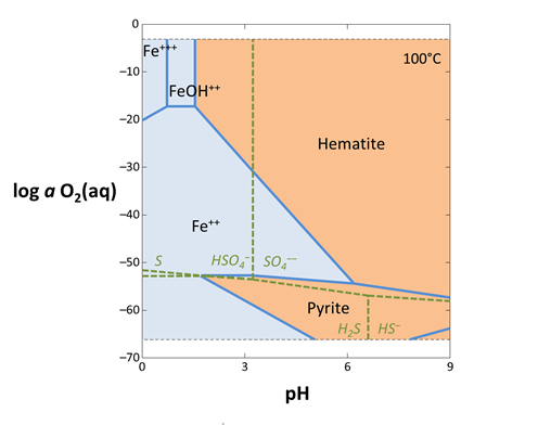
By adding SO42− to our basis set (now Fe++, H+, O2(aq), H2O, and SO42−), we've increased the complexity of our chemical system and enabled the iron-sulfide mineral pyrite (FeS2) to form.
When we check “speciate over x-y”, Act2 divides the calculation into subdiagrams, each in which a single form of sulfur predominates. The dashed lines designate boundaries between the different subdiagrams. You can hover over any field to see the equilibrium species and phase assemblage at that point in a tooltip. You can also toggle the subdiagram boundaries and labels by going to Format → Quick Toggle… and checking or unchecking “mosaic bounds” and “mosaic labels”.
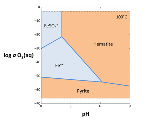
If we had not checked “speciate over x-y” then the diagram would assume sulfur is always present as SO42−, as shown below, even at low pH or oxidation state
Task 2: Stability diagrams
You can diagram stability vs. temperature using Tact. To diagram the thermal stability of calcic aluminosilicates in the presence of quartz, start Tact
and move to the Basis pane.
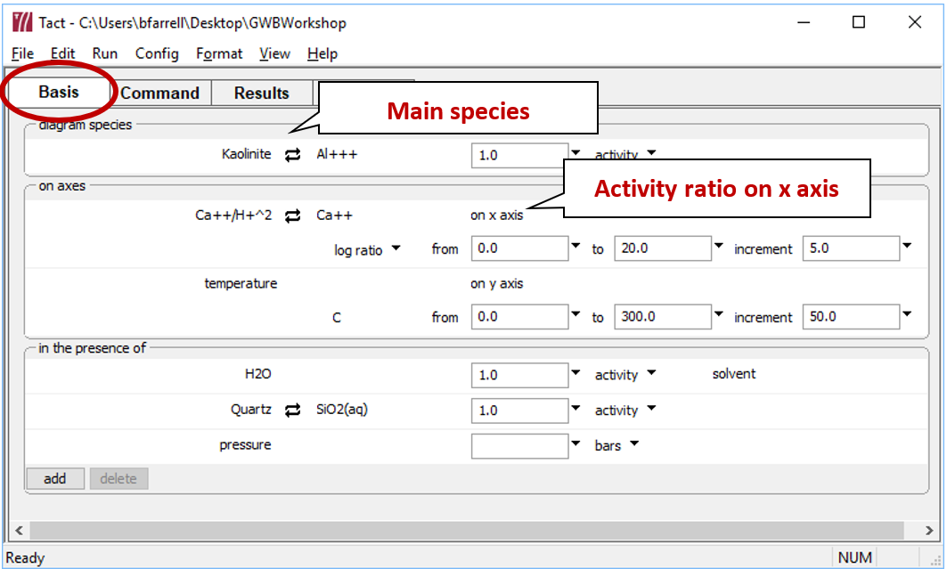
- Under “diagram species” set “Al+++” and then
 Mineral… → “Kaolinite”.
 -
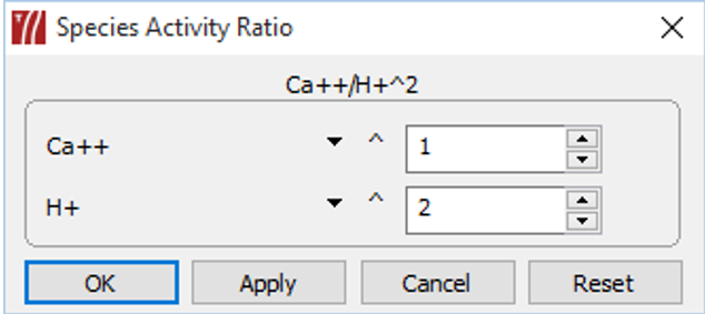
On the x axis, select “Ca++”, then click on Ratio… Set “Ca++” for the numerator, and “H+” squared in the denominator with an exponent of "2".
- Set the axis range from “0” to “20”.
- Under “in the presence of”, add “SiO2(aq)” and swap Mineral… → “Quartz”.
The pane should look like
Move to the Plot pane to view your diagram. Under what conditions are clay minerals stable? Zeolites?
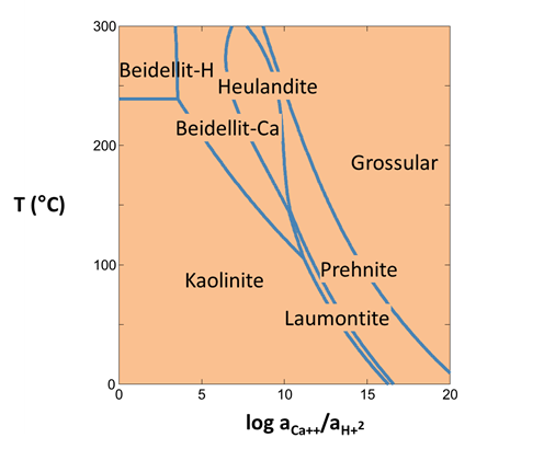
The clay mineral kaolinite predominates over a large portion of the diagram, but is less stable than the beidellite clays at higher temperatures. Of the beidellites, Beidellit-Ca becomes more stable than Beidellit-H at increasing Ca++/H+2 activity ratios. The zeolites Heulandite and Laumontite are stable at higher still ratios.
Task 3: Solubility diagrams
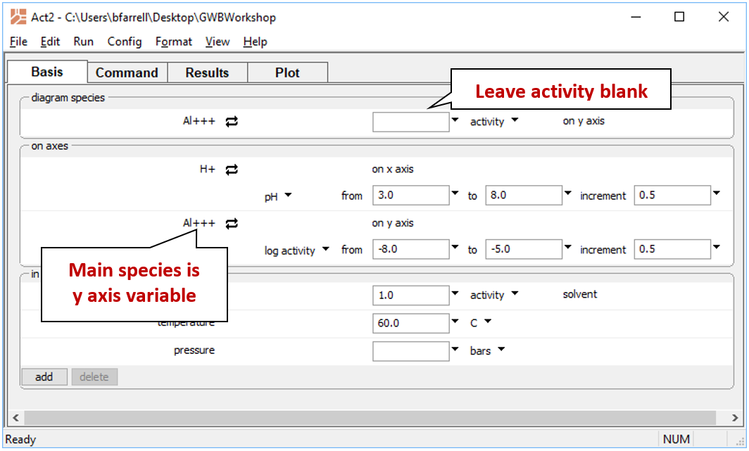
To diagram the solubility of a mineral, open Act2 and set the main species being diagrammed as an axis species. For example, to represent solubility at 60°C in the alumina-water system,
- Under “diagram species”, select “Al+++”.
- Under “on axes”, set “H+” and units of “pH” for x. Set a range from “3” to “8”.
- For the y axis, select “Al+++” and a range from “−8” to “−5”.
- Set “temperature” to 60°C.
The pane should look like
Move to the Plot pane to view your diagram. What kinds of reactions are represented by vertical lines? Horizontal lines?
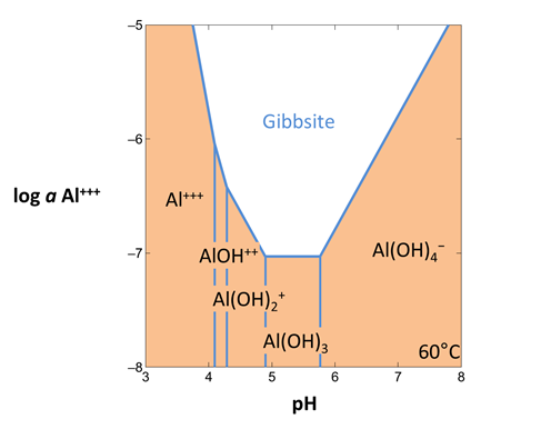
The vertical lines represent protonation or deprotonation of the dissolved aluminum species
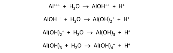
while the horizontal and sloped lines show reactions by which Gibbsite dissolves. Gibbsite is relatively soluble at both the lower and higher pH values shown, but insoluble at intermediate pH.
To diagram the solubility of a less stable alumina mineral, suppress the more stable form. In this way, you prevent Act2 from considering a particular mineral or species while calculating the diagram.
From the Config → Suppress… dialog
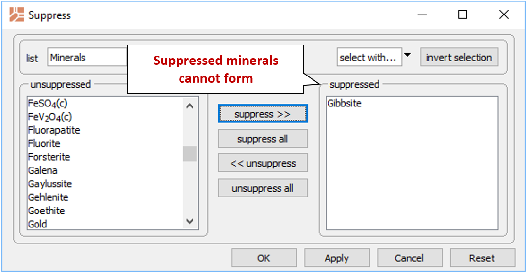
select “Gibbsite” and then suppress >> to prevent it from forming. Take a look at the resulting plot. Suppress “Diaspore” and calculate the diagram once again.
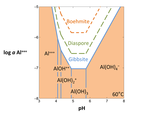
The diagram below shows the three plots assembled together in MS PowerPoint. After suppressing Gibbsite, the less stable (more soluble) mineral Diaspore appears on our diagram. Similarly, after suppressing Diaspore, the more soluble Boehmite appears
Authors
Craig M. Bethke and Brian Farrell. © Copyright 2016–2026 Aqueous Solutions LLC. This lesson may be reproduced and modified freely to support any licensed use of The Geochemist's Workbench® software, provided that any derived materials acknowledge original authorship.
References
Bethke, C.M., B. Farrell, and M. Sharifi, 2026, The Geochemist's Workbench®, Release 18: GWB Essentials Guide. Aqueous Solutions LLC, Champaign, IL, 232 pp.
Comfortable with stability diagrams?
Move on to the next topic, Reactions and Equilibrium Lines, or return to the GWB Online Academy home.