
Reactions and equilibrium lines
Reactions and Equilibrium Lines is part of a free web series, GWB Online Academy, by Aqueous Solutions LLC.
What you need:
- GWB Essentials recommended
Download this unit to use in your courses:
- Lesson plan (.pdf)
- PowerPoint slides (.pptx)
Introduction
The Eh-pH diagram below was created using Act2. The dashed lines that limit the top and bottom of the plot show the stability limits of water at 1 atmosphere pressure. The diagram shows various aqueous species, minerals, and gases that are predominant under the chosen conditions
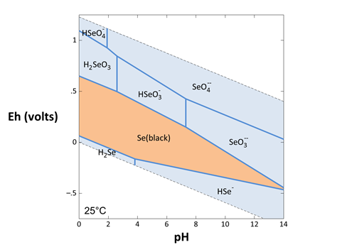
Each solid line on the diagram represents a reaction between species at equilibrium. You can use Rxn to find the stoichiometry of any reaction, as well as the equation for the equilibrium line, as described in the task below.
If you'd like to create the diagram yourself using Act2, click “show instructions” below, or visit the Stability Diagrams section for more information. Otherwise, proceed to the first task to get started with Rxn.
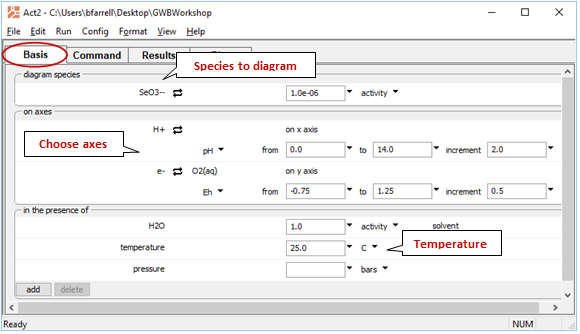
Act2 calculates geochemical stability diagrams on activity or fugacity coordinates. To calculate an Eh-pH diagram for selenium, for example, start the program and move to the Basis pane:
- Under “diagram species”, click on “???” and select “SeO3−−”. Set activity to “10^-6”.
- Under “on axes”, for “on x axis” click on “???” and select “H+”. Change the unit from “log activity” to “pH”. The axis automatically spans from 0 to 14, but you can adjust the range.
- For “on y axis”, click on “???” and select “O2(aq)”. Click on the swap button
 next to the basis entry for “O2(aq)” and select Aqueous…→ e−. Change the unit from “log activity” to “Eh”.
The pane should look like this:
Move to the Plot pane to view your diagram.
Task 1 - Reactions and equilibrium lines
In Rxn you set a species, mineral, or gas to appear on the left side of the reaction, and swap the basis to pull in the various species you want to appear in the reaction.
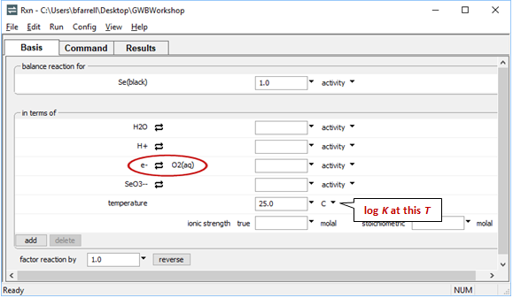
To show the reaction by which elemental selenium is oxidized to SeO32−, start Rxn and under “balance reaction for”, select “???” → Mineral… → Se(black). Set “temperature” to 25°C
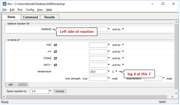
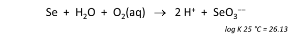
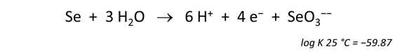
Move to the Results pane and click Run. What is the resulting chemical reaction and log K?
Now let's balance the corresponding half-cell reaction. Click on the swap button next to the basis entry for “O2(aq)” and select Aqueous… → e−
Move to the Results pane and click Run. How has the reaction changed?
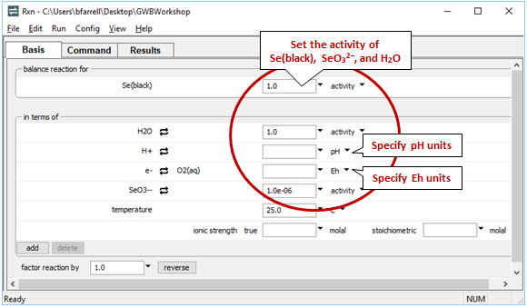
Rxn will also produce a general equilibrium equation written in terms of the activity of species in the reaction. Returning to the Basis pane, let's set some constraints to match those set in our diagram. The activity of a mineral like Se(black) defaults to 1, and we'll set the activity of SeO32− to 10−6 and the activity of H2O to 1. Finally, we'll specify Eh and pH units
Return to the Results pane and click Run. After clicking the “+” to view more output, find the equilibrium equation at the bottom
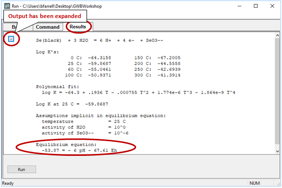
Can you find where this line plots on your Eh-pH diagram? What happens to the line's position if you change the activity of SeO32−?
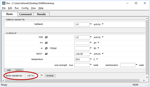
You can simplify the reaction and equilibrium equation further by setting a factor
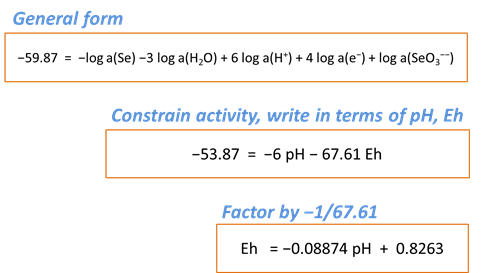
To do so, set “factor reaction by” on the Basis pane
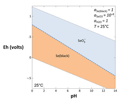
The line is plotted below:
By manipulating Rxn's Basis pane, you can write reactions between any pair of species. You can do so by setting a new species to appear on the left side of the reaction (the “balance reaction for” species), or by swapping out any of the species under “in terms of”.
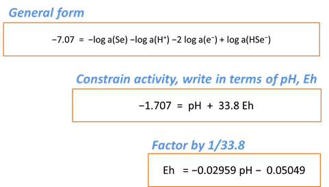
To write the reaction between elemental selenium and HSe−, for example, click on the swap button next to “SeO3−−” and select Aqueous… → “HSe−”. The Basis pane should look like this
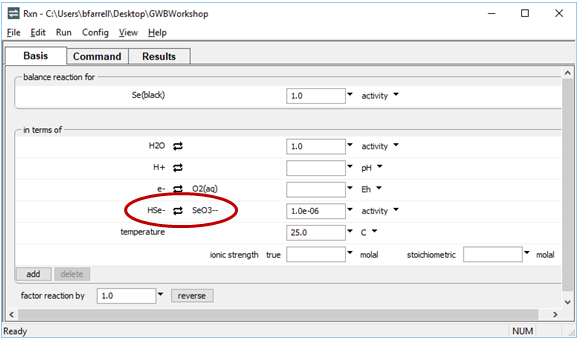
Move to the Results pane and click Run. Rxn will have generated a new reaction and equilibrium equation.
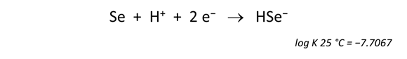
You can factor the reaction like before
The second equation is plotted below with the equation for the first reaction
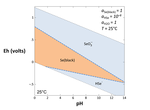
By repeating this procedure to determine the equilibrium equation for all possible reactions between selenium species, you could assemble all of the equilibrium lines on one set of axes to create an activity diagram
The process of calculating diagrams by hand becomes cumbersome as the numbers of species considered increases. The amount of work involved, in fact, rises quadratically because there are n x (n − 1) / 2 reactions among n species. In a system of 100 aqueous species and minerals, for example, there are about 5000 possible reactions. Fortunately, we can let the computer do the work by using Act2, as we've already seen.
Authors
Craig M. Bethke and Brian Farrell. © Copyright 2016–2026 Aqueous Solutions LLC. This lesson may be reproduced and modified freely to support any licensed use of The Geochemist's Workbench® software, provided that any derived materials acknowledge original authorship.
References
Bethke, C.M., 2022, Geochemical and Biogeochemical Reaction Modeling, 3rd ed. Cambridge University Press, New York, 520 pp.
Bethke, C.M., B. Farrell, and M. Sharifi, 2026, The Geochemist's Workbench®, Release 18: GWB Essentials Guide. Aqueous Solutions LLC, Champaign, IL, 232 pp.
Comfortable with reactions and equilibrium lines?
Move on to the next topic, Equilibrium Models, or return to the GWB Online Academy home.