
Mass transport
Mass Transport is part of a free web series, GWB Online Academy, by Aqueous Solutions LLC.
What you need:
- GWB Professional recommended
-
Input file:
 Pulse.x1t
Download this unit to use in your courses:
- Lesson plan (.pdf)
- PowerPoint slides (.pptx)
Click on a file or right-click and select “Save link as…” to download.
Introduction
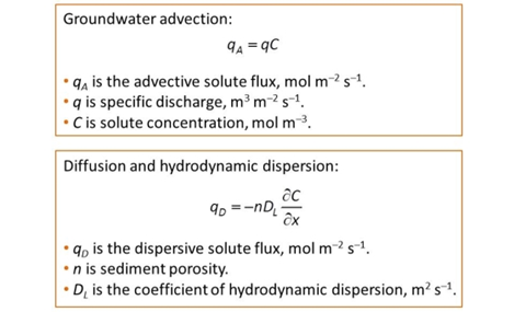
Mass transport is the movement of solutes within a groundwater flow regime. There are several important transport processes:
- Advection—the movement of solutes along with the flowing water
- Hydrodynamic dispersion—results from physical mixing of the flowing groundwater
- Molecular diffusion—arises from Brownian motion of molecules within fluid
We can determine solute fluxes from these processes as follows:
Task 1: Migration of a non-reacting contaminant
Let's construct a model of how a contaminant might migrate in flowing groundwater, neglecting for the moment the possibility of chemical reaction.
In our model, inorganic Pb contamination passes into an aquifer. After 2 years, the source is removed and the aquifer is flushed with ambient water.
Double-click on file “Pulse.x1t” and look at the Initial pane in X1t
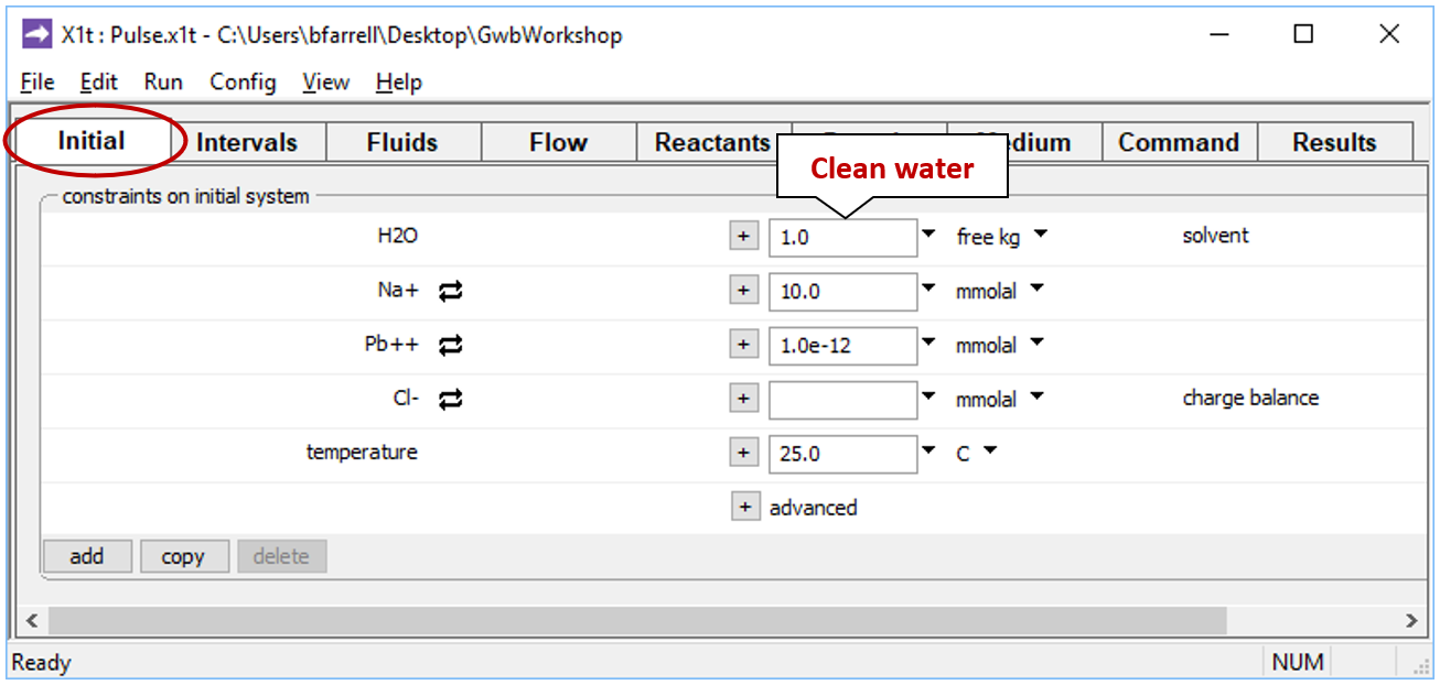
We've specified here that the aquifer be filled initially with clean water.
Moving to the Intervals pane
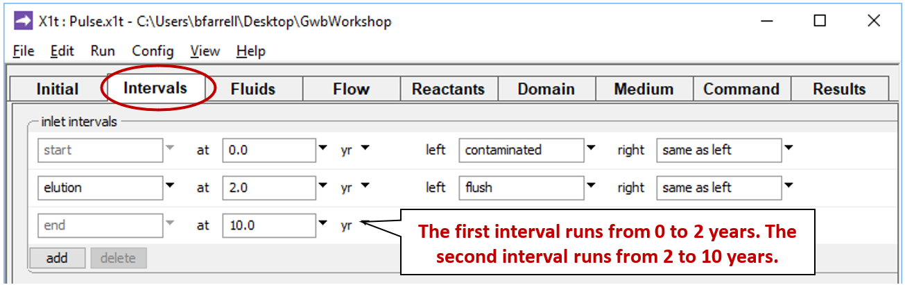
we've set start and end times for two reaction intervals, the imbibition and elution legs of the simulation. We've additionally designated two fluids, “contaminated” and “flush”, to flow into the left side of the domain during the imbibition (start) and elution intervals, respectively.
The Fluids pane contains the two boundary fluids
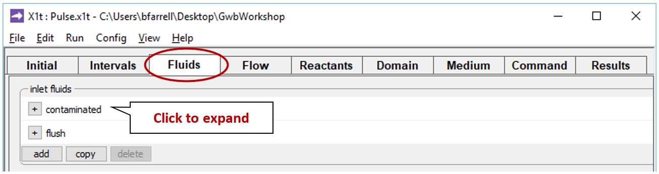
By expanding the  signs, we can view the “contaminated” fluid, which will be introduced in the imbibition leg
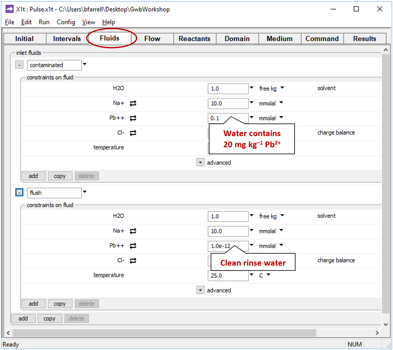
as well as the “flush” fluid: clean rinse water that will flow in during elution.
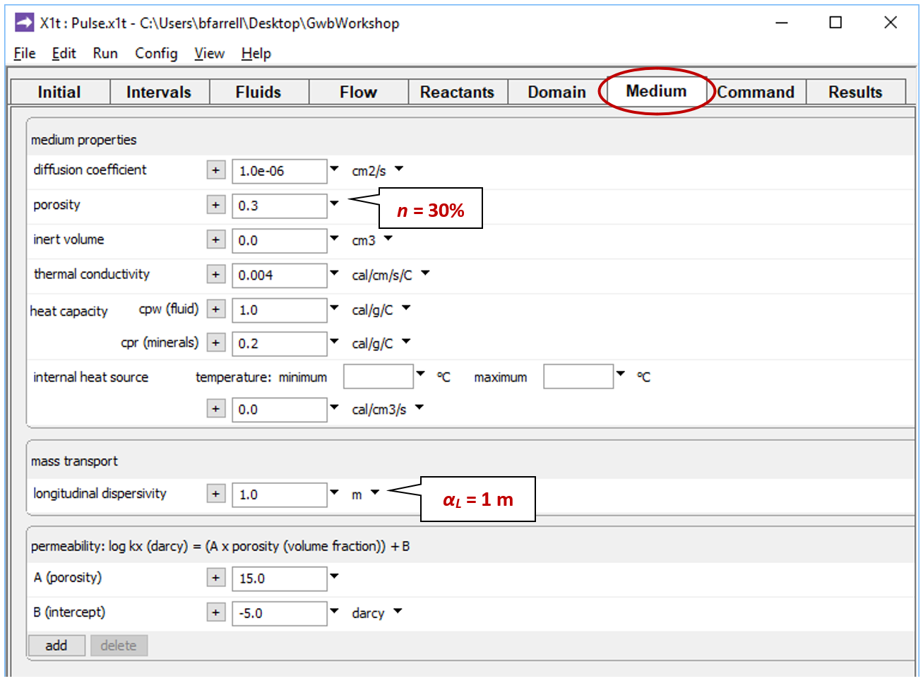
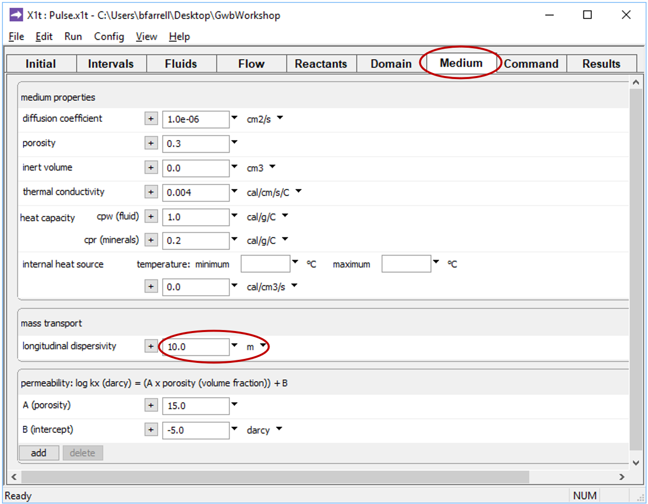
On the Medium pane you can see the values set for porosity and dispersivity
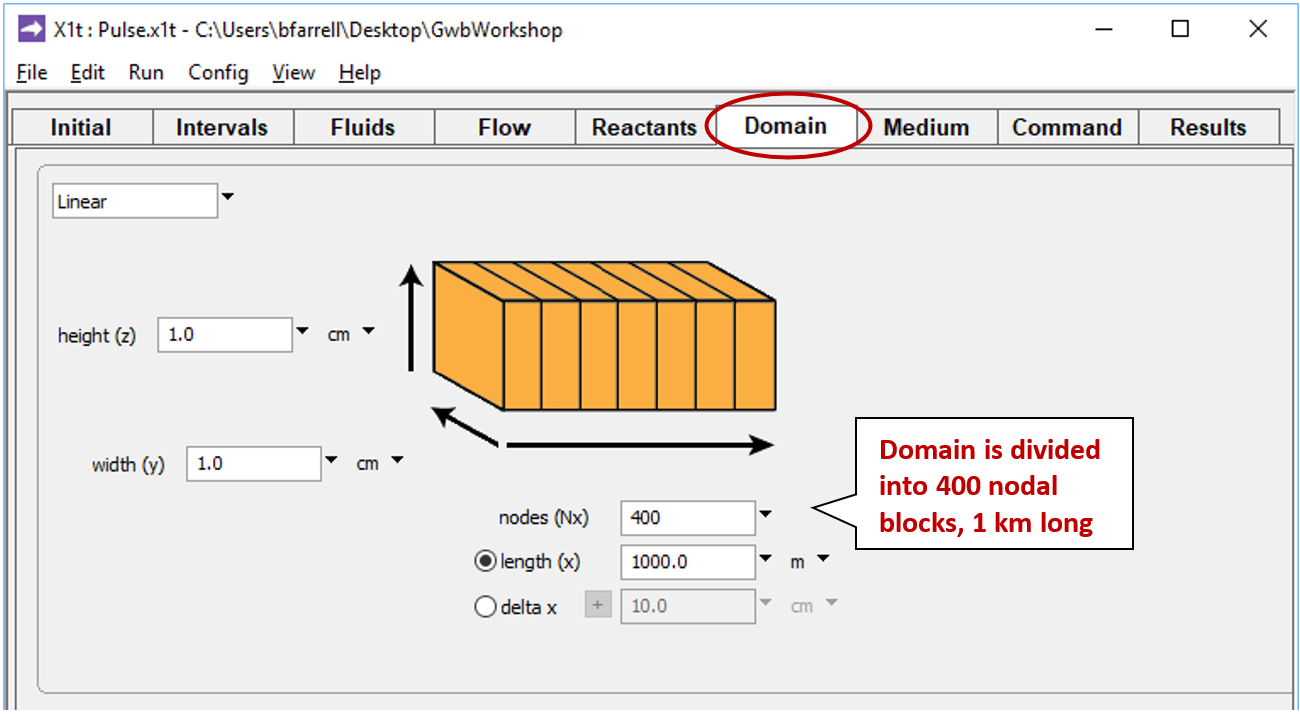
Check the domain size and gridding by moving to the Domain pane
We set the rate at which fluid passes into the domain by moving to the Flow pane
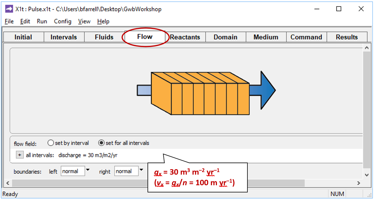
A positive specific discharge indicates that fluid will flow from left to right. The simulation spans 10 years, so given the porosity and discharge values we've set, the fluid in the aquifer will be displaced once over the course of the simulation.
Before launching the run, go to Config → Output... and enter “_pulse” in the suffix field
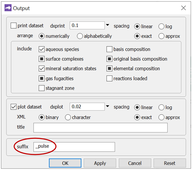
The suffix will be appended to the names of your output datasets, so you can go back to examine the results without rerunning the model. Click OK.
Trigger the calculation by selecting Run → Go. X1t will move to the Results pane, trace the simulation, and when it's done, offer to extend the run
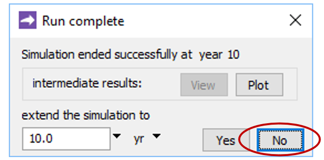
Click No.
Now, look at the bottom of the Results pane
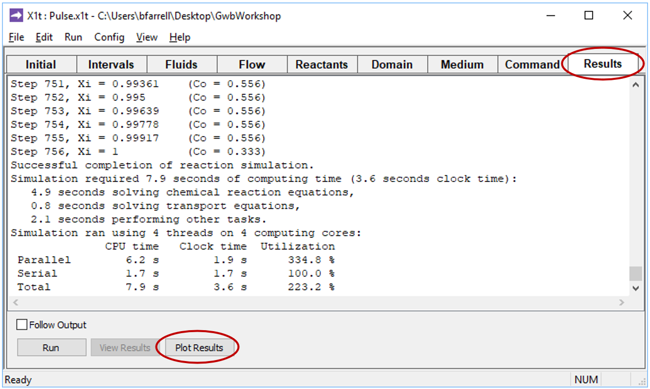
and click on the Plot Results button to launch Xtplot.
Configure the plot as indicated below
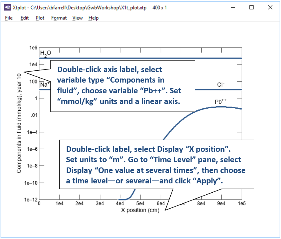
Your diagram should look like this:
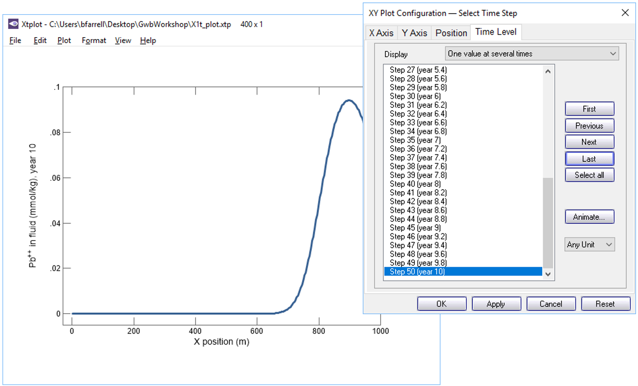
Now, let's animate the plot. On the XY Plot dialog, go to the Y Axis pane and uncheck the “Auto-scale” option
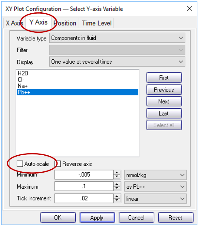
In this way, you hold steady the y-axis range over the animation. Then, on the main window, choose Format → Animate...
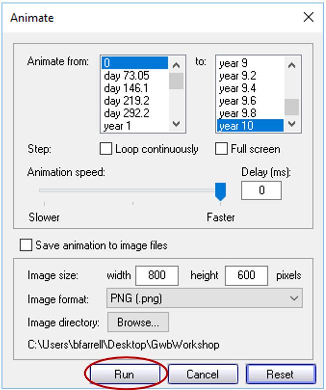
and click on the Run button. How does the shape of the pulse change as it traverses the aquifer from left to right?
We plotted the results after 2, 4, 6, 8 and 10 years of transport and, using MS PowerPoint, assembled them into a single image, shown below
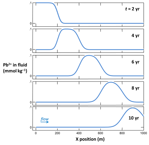
As you can see, the solute pulse is translated from left to right across the domain due to advection. As it migrates, the pulse spreads out and the peak concentration attenuates somewhat due to hydrodynamic dispersion.
Here's a video showing you how to construct the model and plot the results.
More background
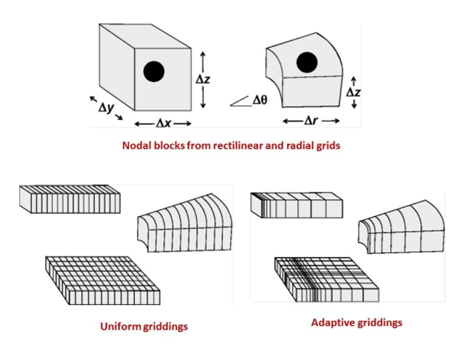
How was our first model solved? The solution to a reactive transport problem is found using the "divide and conquer" strategy. A continuous domain is discretized into a number of nodal blocks, each of which has a single value for porosity, temperature, pH, etc.
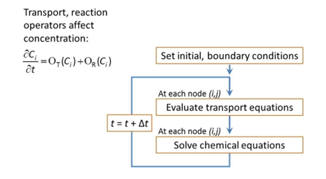
Continuing with the "divide and conquer" strategy, the numerical model uses a technique called “operator splitting” to solve the transport equations separately from the reaction equations.
Now that you have a little more understanding of the numerical solution, let's get back to the physical problem. Specifically, what's the role of dispersion? Look at the illustration below.
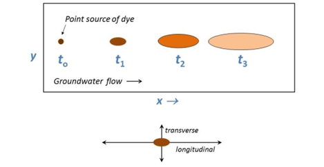
Dispersion results from physical mixing of flowing groundwater. A drop of dye dissolved in the water would spread out as some of the water molecules take more tortuous paths through the aquifer than others.
Task 2: Effects of dispersion
How does dispersion affect contaminant migration? Let's find out.
Go to the Medium pane and change the entry for dispersivity from “1 m” to “10 m”
On Config → Output… set a new suffix “_disp”
Click OK, then on the main window select Run → Go. When X1t finishes, launch Xtplot to render the results. Compared to the first model, how have the results changed?
The most recent results, in green, are plotted along with our results from the previous calculation
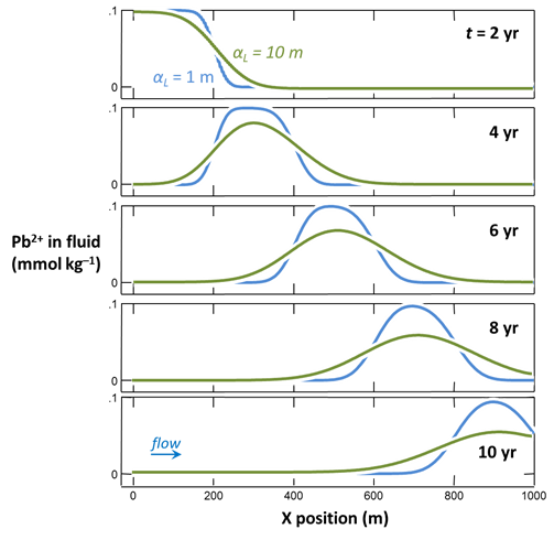
By increasing the dispersivity value, we prescribe a higher coefficient of hydrodynamic dispersion. As a result, the solute pulse broadens significantly as some solute moves ahead of the average groundwater flow, and some lags behind it. With greater dispersion, attenuation of the pulse from dispersive mixing becomes apparent.
You can compare side-by-side instances of Xtplot. Double-click on “X1t_plot_pulse.xtp” to render your earlier results. If you feel ambitious, you can build up a composite diagram in MS PowerPoint to show both results in one diagram.
Animation of two-dimensional example
This movie shows the results of X2t simulations of the migration of inorganic Pb through an aquifer. The contaminant, taken in the simulation as non-reactive, leaks into the aquifer over a period of 1 month and is entrained in the flowing groundwater.
The movie shows output from two simulations:
- One in which dispersion is taken as a Fickian process
- A second in which the dispersion arises from heterogeneity prescribed in the aquifer
Authors
Craig M. Bethke and Brian Farrell. © Copyright 2016–2026 Aqueous Solutions LLC. This lesson may be reproduced and modified freely to support any licensed use of The Geochemist's Workbench® software, provided that any derived materials acknowledge original authorship.
References
Anderson, M.P., 1984, Movement of Contaminants in Groundwater. In Groundwater Contamination, National Academy Press, 37–45.
Bethke, C.M., 2022, Geochemical and Biogeochemical Reaction Modeling, 3rd ed. Cambridge University Press, New York, 520 pp.
Bethke, C.M., B. Farrell, and M. Sharifi, 2026, The Geochemist's Workbench®, Release 18: GWB Reactive Transport Modeling Guide. Aqueous Solutions LLC, Champaign, IL, 191 pp.
Freeze, R.A. and J.A. Cherry, 1979, Groundwater. Prentice Hall, Englewood Cliffs, NJ, 604 pp.
Comfortable with mass transport?
Move on to the next topic, Numerical Dispersion, or return to the GWB Online Academy home.