
Sorbing solutes
Sorbing Solutes is part of a free web series, GWB Online Academy, by Aqueous Solutions LLC.
What you need:
- GWB Professional recommended
-
Input files:
 Pulse.x1t,
 Pb-Kd.sdat,
Pb-Freundlich.sdat,
Pb-Kd.sdat,
Pb-Freundlich.sdat,
 Freund2D.x2t
Download this unit to use in your courses:
- Lesson plan (.pdf)
- PowerPoint slides (.pptx)
Click on a file or right-click and select “Save link as…” to download.
Introduction
The distribution coefficient approach—commonly referred to as the Kd approach—is the most widely applied method in environmental geochemistry for predicting the sorption of contaminant species onto sediments. The distribution coefficient Kd itself is simply the ratio under specific conditions of the sorbed to the dissolved mass of a contaminant. In other words,
where S is the sorbed concentration, in moles per gram dry sediment, Kd is the distribution coefficient, in units of cm3 per gram, and C is the solute concentration, in moles per cm3.
The approach implies a reaction such as
By the Freundlich method, another empirical approach,
where Kf is the Freundlich coefficient, and n is the Freundlich exponent, which can range from 0 to 1. The Freundlich approach simply reduces to the linear Kd when the Freundlich exponent is 1.
The figure below shows sorption of selenate to a soil, showing mass sorbed per gram of dry soil, as a function of concentration in solution. Lines are fits to the data using the activity Kd, activity Freundlich, and Langmuir approaches
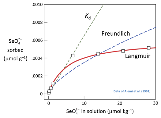
As can be seen, sorption by the Kd approach is equally effective at any concentration, whereas the exponent n in the Freundlich approach predicts progressively less effective sorption as concentration increases.
The activity Kd and activity Freundlich models (also known as reaction Kd and reaction Freundlich) that are coded into geochemical modeling software like The Geochemist's Workbench differ from the general approach:
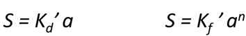
where a is the activity of the free species and Kd' and Kf' account for the ion activity coefficient and ionized fraction of a component. Coefficients calculated in the traditional manner, therefore, need to be corrected by a factor of the species' activity coefficient. Care should be taken to apply them only to systems similar to that for which they were originally determined.
Task 1: Kd approach
In a test, sediment from the aquifer sorbed Pb2+ according to a distribution coefficient Kd of .16 cm3 g–1. The concentration of dissolved lead in the test was about 10 µmolar. Our job is to revise our model of Pb2+ transport in the aquifer to account for sorption.
The activity coefficient for Pb2+ in our groundwater is about .66, and the free ion makes up 80% of dissolved Pb, so the distribution coefficient Kd' for the activity Kd model works out to .30×10–3 mol g–1.
To set up the model, double-click once again on file “Pulse.x1t”. In X1t, go to File → Open → Sorbing Surfaces… (or Config → Sorbing Surfaces…), then navigate to the course directory and select file “Pb-Kd.sdat”, then close the Sorbing Surfaces dialog
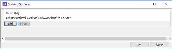
You can confirm you've pulled in the correct value for Kd' by clicking on File → View and selecting “.\Pb-Kd.sdat”.
Now, set “_Kd” as the suffix
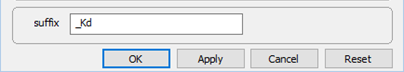
and select Run → Go to trigger the calculation. Graph the results with Xtplot, as before.
How does sorption affect Pb2+ migration in the aquifer? The amount of Pb2+ dissolved in groundwater there?
The plot below shows the results of simulating sorption according to the Kd approach, in green, together with the non-reacting case (in blue)
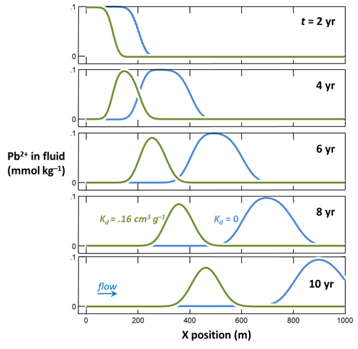
In the Kd case, the pulse is retarded relative to the non-reacting case. The size of the pulse is smaller when sorption is considered because a portion of the contaminant is sorbed to the aquifer, decreasing the concentration in solution.
We can calculate a retardation factor RF
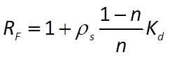
where n is porosity, and ρs is sediment density. Since porosity is 30% in our case, if we take a density of 2.65 g/cm3, the RF is about 2. As you can see from the plot, the pulse migrates at about half the velocity of a non-reacting solute.
Task 2: Freundlich isotherm
Repeating the test using differing amounts of lead, we find Kd varies depending on the Pb2+ concentration. To account for this observation, we fit the test results to a Freundlich isotherm with a Kf' of 9.5×10⁻⁶ and an nf of 0.7. The Freundlich parameterization is equivalent to the Kd approach at a Pb2+ concentration of 10 µmolar.
To run the Freundlich case, return in X1t to the Config → Sorbing Surfaces… dialog. Click on the entry for the “Pb-Kd.sdat” dataset so that it's highlighted, then press the delete key on your keyboard to remove it. Click on  , then read in file “Pb-Freundlich.sdat”
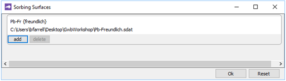
and close the dialog.
Set a suffix “_Freundlich”
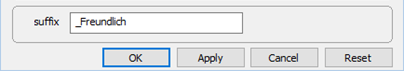
and select Run → Go.
How did adopting a Freundlich isotherm affect the calculation results, compared to when we took the Kd approach to describe sorption?
Results accounting for the Freundlich isotherm are plotted in orange, together with the Kd approach (in green) and the non-reacting case (in blue)
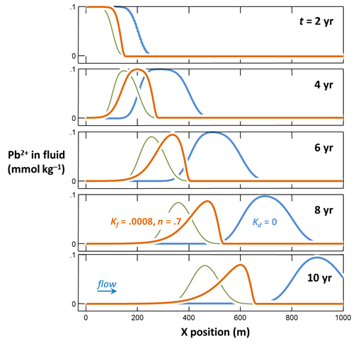
Like the Kd approach, the pulse's migration is retarded. Unlike with the Kd approach, the pulse becomes highly asymmetric, with a steep leading edge and an elongated trailing edge. This is because the effectiveness of sorption depends on the concentration of the ion in solution according to the Freundlich method.
Like in our Dual Porosity model, sorption by the Freundlich approach results in a characteristic tail at the trailing edge of the pulse.
Task 3: Two dimensions
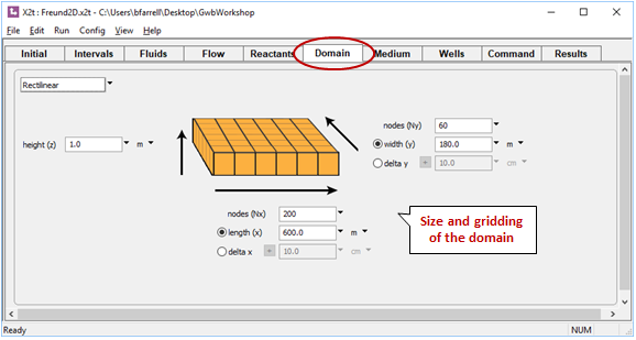
To carry the previous run into two dimensions, start program X2t by double-clicking on file “Freund2D.x2t”. Move to the Domain pane. Here, you can see the domain and how it's discretized
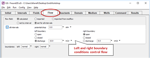
Move to the Flow pane. Here, you can see the boundary conditions for calculating the flow field, which moves from left to right
Move to the Wells pane
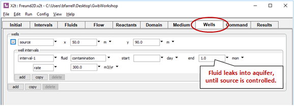
We've positioned a well toward the upstream end of the domain to introduce leakage from the contaminant source. Fluid from the well enters the aquifer during the first month of the simulation.
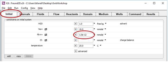
Examine the Initial pane. Here, we've set the aquifer to be filled with clean water initially
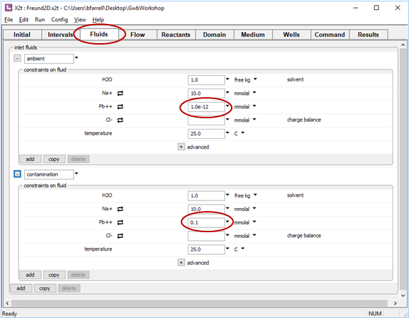
Check as well the Fluids pane. The “ambient” fluid is set to the same composition as the Initial fluid. The “contamination” fluid, in contrast, defines water contaminated with Pb2+
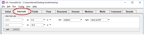
On the Intervals pane, we've associated the clean ambient water with the left side of the domain and set the duration of the simulation to 10 years
On the Medium pane, we've set the properties so that differential flow gives rise to dispersion. Porosity varies in a Gaussian distribution about 30%. The logarithm of permeability varies with porosity, so the permeability field is heterogeneous, too, and the resulting flow field is irregular
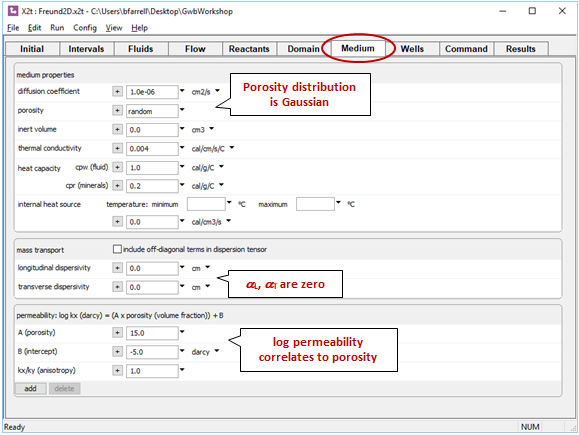
We're not using the Fickian concept of dispersion, so the values set for αL and αT from Fick's law are 0.
You can trace the simulation by selecting Run → Go.
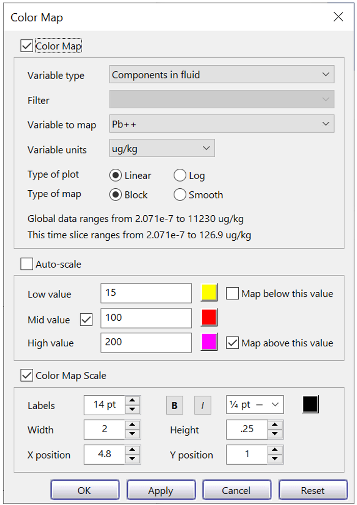
To render the simulation results, click  to launch Xtplot, and select Plot → Map View. Then chose Format → Color Map… , and in the top five fields choose: “Components in fluid”, “blank”, “Pb2+”, “ug/kg”, and “Linear”.
Uncheck “Auto-scale” and map low, mid, and high values to “15 µg/kg”, “100 µg/kg”, and “200 µg/kg”. Now, associate the values with yellow, red, and magenta.
To mask areas of the aquifer where Pb2+ concentration falls below the USEPA's MCL of 15 µg/kg, uncheck “Map below this value”. The program will mask values in the range 0 to 15 µg/kg using the color white. When you're done, the dialog should look like this:
Click OK.
Now, click on Format → Time Step…
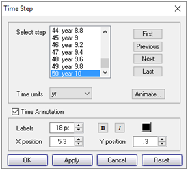
choose a time to render and click Apply. You can move forward and backward in time with the Next and Previous buttons.
Finally, click on  and on the dialog that pops up
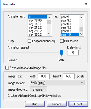
click Run.
Note the “Loop continuously” and “Full screen” check boxes. Note further the “Save animation to image files” check box. We will use this option to save the frames from which we'll make video clips of our animations.
Animation of two-dimensional example
Animations in this movie show a simulation of Pb2+ transport through a heterogeneous medium, accounting for contaminant attenuation by sorption to the aquifer solids. There is a series of three simulations:
- The non-reacting case, for reference
- The lead ion sorbs according to a distribution coefficient Kd
- Sorption follows a Freundlich isotherm
Authors
Craig M. Bethke and Brian Farrell. © Copyright 2016–2026 Aqueous Solutions LLC. This lesson may be reproduced and modified freely to support any licensed use of The Geochemist's Workbench® software, provided that any derived materials acknowledge original authorship.
References
Alemi, M.H., D.A. Goldhamer and D.R. Nelson, 1991, Modeling selenium transport in steady-state, unsaturated soil columns. Journal of Environmental Quality 20, 89–95.
Bethke, C.M., 2022, Geochemical and Biogeochemical Reaction Modeling, 3rd ed. Cambridge University Press, New York, 520 pp.
Bethke, C.M., B. Farrell, and M. Sharifi, 2026, The Geochemist's Workbench®, Release 18: GWB Reactive Transport Modeling Guide. Aqueous Solutions LLC, Champaign, IL, 191 pp.
Comfortable with sorbing solutes?
Move on to the next topic, Surface Complexation, or return to the GWB Online Academy home.