
Dual porosity
Dual Porosity is part of a free web series, GWB Online Academy, by Aqueous Solutions LLC.
What you need:
- GWB Professional recommended
-
Input file:
 Pulse.x1t
Download this unit to use in your courses:
- Lesson plan (.pdf)
- PowerPoint slides (.pptx)
Click on a file or right-click and select “Save link as…” to download.
Introduction
Bypassing is a common problem in environmental hydrology, as it often undermines active remediation strategies. As water flows through an aquifer, it commonly bypasses low conductivity sediments, or stagnant zones. Solute can, however, diffuse into or out of these stagnant zones, depending on the relative concentrations of solute in the high and low conductivity zones of the aquifer.
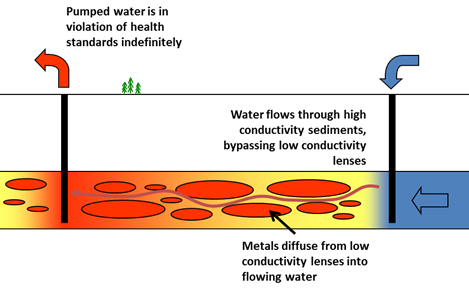
In remediating an aquifer by the pump and treat method, all the produced water comes from the high-conductivity, or free-flowing zones. Clean water flushed through the aquifer can become contaminated as solute diffuses out of the stagnant zones into the water.
A dual porosity model can account for the effects of preferential flow, bypassing, and solute exchange. In the model, each nodal block is divided into free-flowing and stagnant fractions. Water is transported from one node to the next only within the free-flowing fraction. Within a nodal block, however, solute diffuses from the free-flowing fraction into and out of stagnant zones.
The geometry of a stagnant zone can be described by spheres, blocks, or fractures, but the controlling factor is contact area. You set a stagnant fraction Xstag, and radius r or half-width δ of stagnant spheres or blocks. You can also set D*, Nsubnode, δdiff, RF, and so on.
Each nodal block in a dual porosity model, assuming the spherical geometry, looks like this
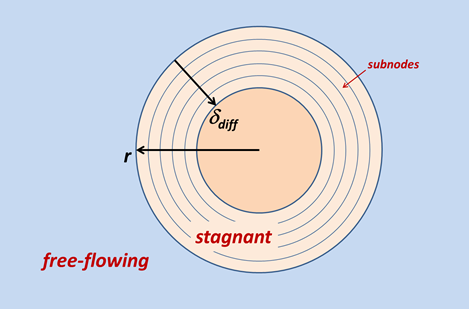
where r is the radius of the stagnant zone. The stagnant fraction and radius set the surface area over which diffusion occurs. The stagnant zone is divided into a number of subnodes extending from the free-flowing zone–stagnant zone interface to the center of the sphere. The diffusion equation is solved along this coordinate, or if the diffusion length δdiff is set, within only the outer skin of the stagnant zone.
Task 1: Dual porosity model of Pb transport
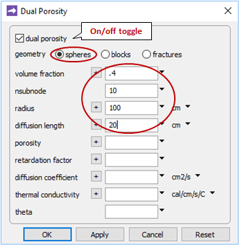
We'll model Pb transport as before, except we'll take 40% of the aquifer to be stagnant. Water is stationary there, but the contaminant can diffuse in from the free-flowing zone, and back out. The stagnant zones in the model have a characteristic radius of 1 meter. In light of the diffusion length  corresponding to a time span of 10 years, we'll trace diffusion within only the zones' outer 20 cm.
Open file "Pulse.x1t". Start the Config → Dual Porosity… dialog and configure the dual porosity feature as shown
Click OK. Set a suffix "_dual" (Config → Output…)
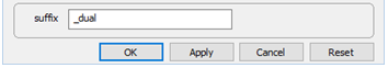
and click OK. Click on Run → Go to execute the simulation, then render the results with Xtplot. How do they differ from a single porosity simulation?
The results below compare the dual porosity simulation with a uniform, or single porosity, medium like that described in the Mass Transport section. In the dual porosity model, the pulse migrates through the domain more quickly than in the uniform case. The pulse is attenuated near its leading edge as solute diffuses into the stagnant zone
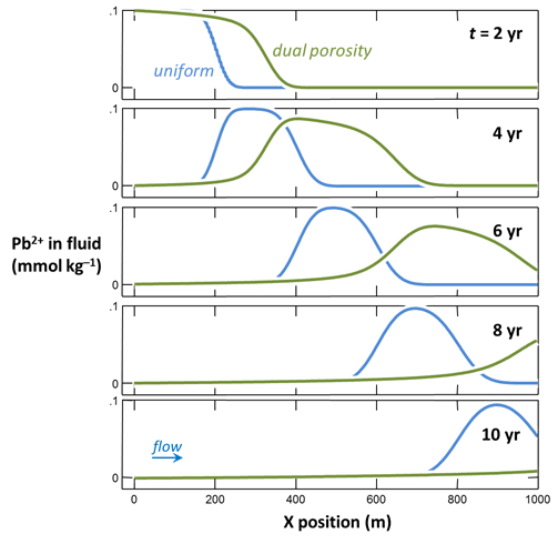
The trailing edge of the pulse exhibits tailing; the Pb++ concentration is higher than in the uniform case because as clean water flushes the aquifer, the solute diffuses back out of the stagnant zone.
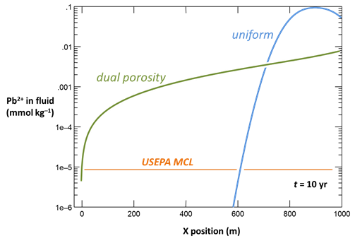
By plotting concentration on a log scale, it becomes readily apparent that after 10 years of pumping, the Pb++ concentration is at least 10 times the EPA Maximum Contaminant Level (MCL) almost everywhere in the domain
Here's a video of the X1t setup
Animation of two-dimensional example
This movie shows the results of X2t simulations of the migration of inorganic Pb through an aquifer. A dual porosity model accounts for diffusion into and out of stagnant zones in the aquifer. There are three simulations:
- A single porosity model for a uniform medium, for reference
- A dual porosity simulation in which stagnant zones with a characteristic dimension of 1 m occupy 40% of the aquifer
- The dual porosity model above, applied to a heterogeneous aquifer
Authors
Craig M. Bethke and Brian Farrell. © Copyright 2016–2026 Aqueous Solutions LLC. This lesson may be reproduced and modified freely to support any licensed use of The Geochemist's Workbench® software, provided that any derived materials acknowledge original authorship.
References
Bethke, C.M., B. Farrell,and M. Sharifi, 2026, The Geochemist's Workbench®, Release 18: GWB Reactive Transport Modeling Guide. Aqueous Solutions LLC, Champaign, IL, 191 pp.
Comfortable with dual porosity models?
Move on to the next topic, Sorbing Solutes, or return to the GWB Online Academy home.