
High-salinity fluids
High-Salinity Fluids is part of a free web series, GWB Online Academy, by Aqueous Solutions LLC.
What you need:
- GWB Essentials recommended
-
Input file:
 SebkhatElMelah.gss
Download this unit to use in your courses:
- Lesson plan (.pdf)
- PowerPoint slides (.pptx)
Click on a file or right-click and select “Save link as…” to download.
Introduction
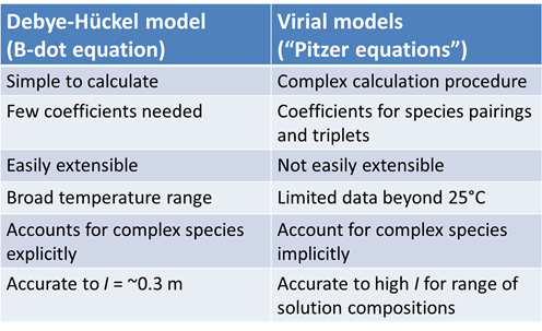
Among the most vexing tasks for geochemical modelers, especially when they work with concentrated solutions, is estimating values for the activity coefficients of electrolyte species. The virial equations offer a conceptual alternative to the standard Debye-Hückel methods for calculating electrolyte activities. Virial methods are frequently employed in geochemical modeling because they can be applied with accuracy at high ionic strength. The table below lists some of the pros and cons of the two approaches.
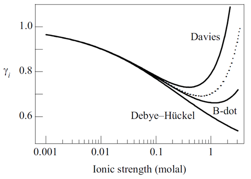
The Debye-Hückel equation gives the activity coefficient of an ion with electrical charge zi and ion size parameter åi. It is notable in that it predicts a species' activity coefficient using only two numbers ( zi and åi) to account for the species' properties and a single value, ionic strength I, to represent the solution. As such, it can be applied readily to study a variety of geochemical systems. Debye-Hückel activity coefficients approach unity when ionic strength nears 0. With increasing ionic strength, the coefficient decreases monotonically.
The Davies equation is a variant of the Debye-Hückel equation that can be carried to somewhat higher ionic stengths. The Davies equation does not decrease monotonically with ionic strength, as the Debye-Hückel equation does. Beginning at ionic strengths of about 0.1 molal, it deviates above the Debye-Hückel function, and at about 0.5 molal starts to increase in value. The Davies equation is reasonably accurate to an ionic strength of about 0.3 or 0.5 molal.
The B-dot equation is widely applied in geochemical models designed to operate over a range of temperatures. The equation is considered reasonably accurate in predicting the activities of Na+ and Cl− ions to concentrations as large as several molal, and of other species to ionic strengths up to about 0.3 to 1 molal.
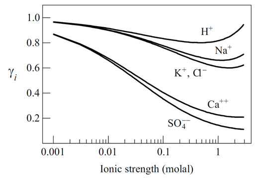
The figure below shows the activity coefficients predicted by the B-dot equation at 25°C for species of differing charge and ion size.
Virial coefficients offer a conceptual alternative to the Debye-Hückel methods for calculating electrolyte activites. One of the most useful implementations for geochemical modeling, published by Harvie et al. (1984), is known as the Harvie-Møller-Weare (or H-M-W ) method. This method treats solutions in the Na-K-Mg-Ca-H-Cl-SO4-OH-HCO3-CO3-CO2-H2O system at 25°C.
The figure below shows the differences in gypsum (CaSO4·2H2O) solubility as a function of NaCl concentration, as calculated by the two methods.
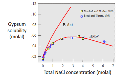
The H-M-W calculations closely coincide with the experimental data, reflecting the fact that that these same data were used in parameterizing the model (Harvie and Weare, 1980). The B-dot results coincide closely with the data only at NaCl concentrations less than about 0.5 molal. At 3 molal concentration, the predicted solubility is about double the measured value.
Task 1: Brine deposits at Sebkhat el Melah
As a test of our ability to calculate activity coefficients in natural brines, we consider groundwater from the Sebkhat el Melah brine deposit near Zarzis, Tunisia (Perthuisot, 1980). The deposit occurs in a buried evaporate basin composed of halite (NaCl), anhydrite (CaSO4), and dolomite [CaMg(CO3)2].
Since the deposit contains halite and anhydrite, the brines should be saturated with respect to these minerals and hence provide a good test of the activity models. The table below contains analyses of brine samples from the deposit. Note the reported pH values are almost certainly incorrect because pH electrodes do not respond accurately in concentrated solutions. Hence, there is little to be gained by calculating dolomite saturation.
To model the brine, we'll need to set the activity model and specify the chemical composition of one of our fluids. To get started, double-click on “SebkhatElMelah.gss”
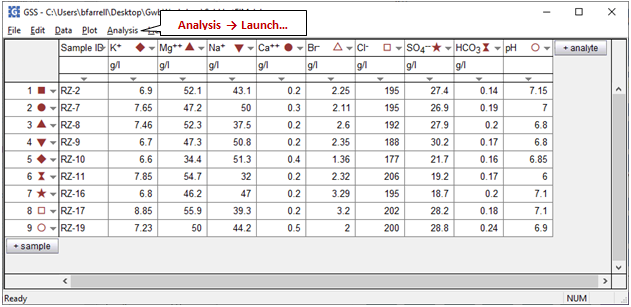
to open a GSS spreadsheet of analyses for 9 brine samples from the deposit. We'll use SpecE8 to figure the distribution of species in the first sample, RZ-2, which allows us to determine the saturation state of halite and anhydrite in the fluid.
Launch SpecE8 directly from GSS by selecting Analysis → Launch…. Choose SpecE8 as the app to launch, select sample RZ-2, then enter the command “balance on Cl-” in the “Trailer commands:” section. The command causes SpecE8 to adjust the concentration of the Cl− component where necessary to maintain charge balance
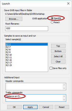
Click Apply.
SpecE8 will open in a separate window. The Basis pane shows the fluid composition of the sample you've chosen
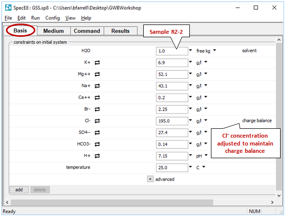
Since we've launched SpecE8 from GSS, SpecE8 used the thermo dataset loaded in GSS. By default, the GWB programs load “thermo.tdat”, a compilation from Lawrence Livermore National Lab that uses the B-dot equation for calculating activity coefficients.
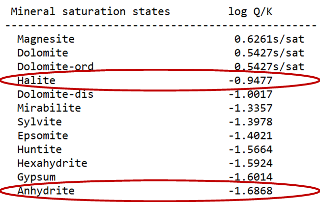
On the Results pane, click View Results to open the text file containing the species' distributions and mineral saturation states predicted by the model.
What is the ionic strength of the fluid? What is the saturation index of halite? Anhydrite? Do they appear to be at equilibrium with the fluid?
Various properties of the fluid can be found at the top of the printed output file, or as Chemical or Physical parameters within the plotting apps. We find that the ionic strength of the fluid is about 6 molal, well outside the range over which the Debye-Hückel (B-dot) method was calibrated
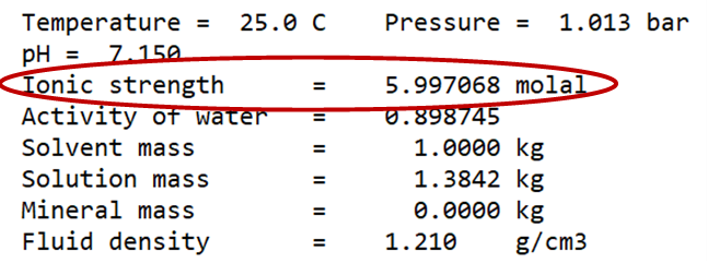
Unsurprisingly, the method predicts that halite and anhydrite are significantly undersaturated in the brine sample
Repeat the calculation using the H-M-W model. In SpecE8, go to File → Open → Thermo Data… and select “thermo_hmw.tdat”. You can view the contents of the dataset by going to File → View → .\thermo_hmw.tdat.
As you can see, the H-M-W model does not account for bromide, so you'll need to remove Br− before performing the calculation
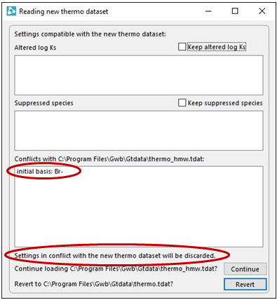
Click Continue on the dialog that pops up to load the new thermo dataset. This action will also remove Br− from consideration.
Go to Config → Output… and append “_hmw” to the suffix before rerunning the simulation.
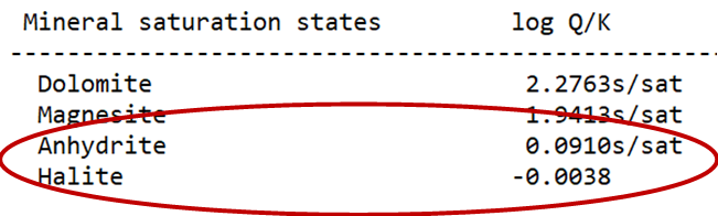
Return to the Results pane, click Run and then View Results. Are the saturation indices for halite and anhydrite significantly different from those calculated earlier? As calculated with the H-M-W model, does this fluid appear to be close to equilibrium with either mineral?
The H-M-W model predicts that halite and anhydrite are near equilibrium with the brine, as we would expect
As usual, we cannot determine whether the remaining discrepancies result from analytical error, error in the activity model, or error from other sources.
Now that we've seen how SpecE8 calculates saturation indices, let's analyze the rest of our samples the fast way: directly within GSS.
Return to GSS and click on File → Open → Thermo Data… → “thermo_hmw.tdat”. The program will load the “thermo_hmw.tdat” dataset to perform our calculations using the virial equations.
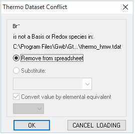
Br− is not included in “thermo_hmw.tdat”, so a warning will appear asking you to remove the entry from your spreadsheet. Click OK
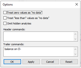
Go to Analysis → Options… and note that the command we entered earlier, “balance on Cl-”, has been retained as a constraint on the calculation
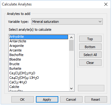
To perform the calculations, click on  → Calculate with SpecE8…, then for “Variable type”, choose “Mineral saturation”, then select “Anhydrite” and “Halite” and click Apply
GSS, teaming in the background with SpecE8, will calculate the saturation state of the two minerals, using the H-M-W activity model.
Are all of the samples in the datasheet close to equilibrium with halite and anhydrite?
The figure below shows saturation indices of several brine samples with respect to halite (left) and anhydrite (right), calculated using the B-dot (in blue) and Harvie-Møller-Weare (in green) models
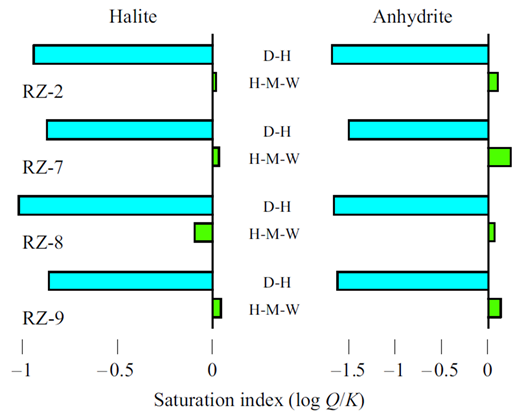
While the B-dot model predicts that both minerals are significantly undersaturated in the brine samples, the H-M-W model predicts they are near equilibrium with the brine, as we would expect.
Authors
Craig M. Bethke and Brian Farrell. © Copyright 2016–2026 Aqueous Solutions LLC. This lesson may be reproduced and modified freely to support any licensed use of The Geochemist's Workbench® software, provided that any derived materials acknowledge original authorship.
References
Bethke, C.M., 2022, Geochemical and Biogeochemical Reaction Modeling, 3rd ed. Cambridge University Press, New York, 520 pp.
Bethke, C.M., B. Farrell, and M. Sharifi, 2026, The Geochemist's Workbench®, Release 18: GWB Essentials Guide. Aqueous Solutions LLC, Champaign, IL, 232 pp.
Block, J. and O.B. Waters, Jr., 1968, The CaSO4-Na2SO4-NaCl-H2O system at 25°C to 100°C. Journal of Chemical and Engineering Data 13, 336–344.
Harvie, C.E., N. Møller and J.H. Weare, 1984, The prediction of mineral solubilities in natural waters, the Na-K-Mg-Ca-H-Cl-SO4-OH-HCO3-CO3-CO2-H2O system to high ionic strengths at 25°C. Geochimica et Cosmochimica Acta, 48, 723–751.
Harvie, C.E. and J.H. Weare, 1980, The prediction of mineral solubilities in natural waters, the Na-K-Mg-Ca-Cl-SO4-H2O system from zero to high concentration at 25°C. Geochimica et Cosmochimica Acta, 44, 981–997.
Marshall, W.L. and R. Slusher, 1966, Thermodynamics of calcium sulfate dehydrate in aqueous sodium chloride solutions, 0-110°C. The Journal of Physical Chemistry, 70, 4015–4027.
Perthuisot, J.P., 1980, Sebkha el Melah near Zarzis: a recent paralic salt basin (Tunisia). In G. Busson (ed.), Evaporite Deposits, Illustration and Interpretation of Some Environmental Sequences, Editions Technip, Paris, pp. 11–17, 92–95.
Comfortable with high salinity models?
Move on to the next topic, Editing Thermo Data, or return to the GWB Online Academy home.