Reactive transport model

Reactive Transport Model is part of a free web series, ChemPlugin Modeling with Python, by Aqueous Solutions LLC.

---

Interface

---

Introduction

In this final example, we culminate our modeling exercises by creating a one-dimensional model of polythermal reactive transport out of ChemPlugin instances. We ask the user to point to an input file of configuration commands. The commands constrain the chemistry of the inlet fluid, as well as the domain's initial chemistry. The input file looks like:

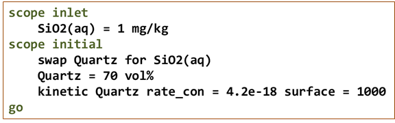
Configuration commands following a “scope inlet” statement apply to the inlet fluid, whereas those following “scope initial” are used to constrain the chemistry of the domain.

The client's output strategy is to write blocks of the calculation results in “print format” to a file “RTM.txt”. Initially, the client writes blocks describing the inlet fluid and the initial state of each of the ChemPlugin instances comprising the domain. Then, every so often over the course of the time marching, the client scans across the domain, writing a block of output for each of the ChemPlugin instances.

To get started, right-click on RTM1.py and open it in Notepad++.

Function “write_results()” writes out the calculation results for each instance in the domain, once every “gap” years:

    from ChemPlugin import *
    import sys

    def write_results(cp, gap, then):
        now = cp[0].Report1("Time", "years")
        if (then - now) < gap / 1e4:
            for i in range(len(cp)):
                cp[i].PrintOutput("RTM.txt", "Instance " + str(i))
            then += gap
        return then

    def end_run(code):
        input("Done!")
        sys.exit(code)

    print("Model reactive transport in one dimension\n")
                

The function employs the “PrintOutput()” member function to trigger output events.

We query the user for the name of an input file and open an input stream from that file.

    # Query user for input file
    while True:
        filename = input("Enter RTM input script: ")
        try:
            inputf = open(filename, 'r')
        except:
            print("The input file named " + filename + " doesn't exist")
        else:
            break
                

The simulation parameters define a domain 100 m x 1 m x 1 m, composed of 100 ChemPlugin instances of 1 m³ each. Rather than setting porosity explicitly, we will query the first ChemPlugin instance in the domain for the value, once it is configured and initialized.

    # simulation parameters
    nx = 100                      # number of instances along x
    length = 100.0                # m
    deltax = length / nx          # m
    deltay = 1.0                  # m
    deltaz = 1.0                  # m
    time_end = 10.0               # years
    delta_years = time_end / 5.0  # years
    next_output = 0.0             # years
                

The simulation is set to span 10 years, writing output at 0 years, and then every 2 years.

To create the ChemPlugin instances that will comprise the model, we, as in previous models, instantiate an instance “cp_inlet” to represent the inlet fluid, and “nx” instances to make up the interior of the domain.

    # Create the inlet and interior instances
    cp_inlet = ChemPlugin()
    cp_inlet.Console("stdout")

    cp = [ChemPlugin() for i in range(nx)]
    cp[0].Console("stdout")
    cp[0].Config("pluses = banner")

    cmd = "volume = " + str(deltax * deltay * deltaz) + " m3; "
    cmd += "time end = " + str(time_end) + " years"

    for c in cp:
        c.Config(cmd)
                

For each of the interior instances, we pass a set of configuration commands that set the instance's bulk volume and the end time of the simulation.

Next, we configure the chemical state of each ChemPlugin instance.

    # Configure inlet, initial domain
    scope = 0
    for line in inputf:
        if line.split() == ["go"]:
            break
        elif line.split() == ["scope", "inlet"]:
            scope = 1
        elif line.split() == ["scope", "initial"]:
            scope = 2
        elif scope == 1:
            cp_inlet.Config(line)
        elif scope == 2:
            for c in cp:
                c.Config(line)
                

The client scans through the input file, sending lines following an occurrence of “scope inlet” to configure “cp_inlet”, and lines after “scope initial” to each of the interior instances.

Once the ChemPlugin instances are configured, the client initializes them with member function “Initialize()”, and writes the boundary and initial conditions to output file “RTM.txt”.

    # Initialize the inlet and interior instances; write out initial conditions
    if cp_inlet.Initialize():
        print("Inlet failed to initialize")
        end_run(-1)

    cp_inlet.PrintOutput("RTM.txt", "Inlet fluid")

    for c in cp:
        if c.Initialize():
            print("Interior instance failed to initialize\n")
            end_run(-1)

    next_output = write_results(cp, delta_years, next_output)
                

To describe mass transport and heat transfer among the instances, the client calculates the flow rate Q, in m³ s⁻¹; the mass transmissivity τ, in the same units; and the thermal transmissivity τ_T, in W K⁻¹.

    # Query user for velocity; calculate flow rate and transmissivities
    veloc_in = float(input("Please enter fluid velocity in m/yr: "))

    velocity = veloc_in / 31557600.                         # m/s
    porosity = cp[0].Report1("porosity")                    # unitless
    flow = deltay * deltaz * porosity * velocity            # m3/s

    diffcoef = 1e-10                                        # m2/s
    dispersivity = 1.0                                      # m
    dispcoef = velocity * dispersivity + diffcoef           # m2/s
    trans = deltay * deltaz * porosity * dispcoef / deltax  # m3/s

    tcond = 2.0                                             # W/m/K
    ttrans = deltay * deltaz * tcond / deltax               # W/K
                

The first two values depend on the flow velocity, v_x, which the client prompts the user to provide, and the porosity n, determined by querying the first instance in the domain.

The code for linking the instances into a flow domain

    # Link the instances
    link = cp[0].Link(cp_inlet)
    link.FlowRate(flow, "m3/s")
    link.Transmissivity(trans, "m3/s")
    link.HeatTrans(ttrans, "W/K")

    for i in range(1, nx):
        link = cp[i].Link(cp[i - 1])
        link.FlowRate(flow, "m3/s")
        link.Transmissivity(trans, "m3/s")
        link.HeatTrans(ttrans, "W/K")

    link = cp[nx - 1].Link()
    link.FlowRate(-flow, "m3/s")
                

parallels the coding used earlier in the diffusion example. In this client, however, we specify transmissivities for both mass transport and heat transfer.

The time marching loop

    # Time marching loop.
    while True:
        deltat = 1e99
        for c in cp:
            deltat = min(deltat, c.ReportTimeStep())
        for c in cp:
            if c.AdvanceTimeStep(deltat): end_run(0)
        span class="blue">for c in cp:
            if c.AdvanceTransport(): end_run(-1)
        span class="blue">for c in cp:
            if c.AdvanceHeatTransport(): end_run(-1)
        span class="blue">for c in cp:
            if c.AdvanceChemical(): end_run(-1)

        next_output = write_results(cp, delta_years, next_output)
                

sets out the sequential computation of mass transport, heat transfer, and chemical reaction.

---

Task 1: Running a reactive transport model

Rather than hard-code the chemical system into the source code of the client program, we can read in a simple input file, like “Infilter.cpi”, shown below:

Configuration commands following a “scope inlet” statement apply to the inlet fluid, whereas those following “scope initial” are used to constrain the chemistry of the domain. The file describes the reaction of dilute water infiltering into a quartz aquifer, where the reaction proceeds according to a kinetic rate law.

To get started, double-click on the RTM1.py file to run it. The Command prompt will launch and prompt you to load an input script for the client.

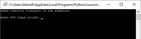
Type “infilter.cpi” and hit Enter.

The client initializes ChemPlugin instances representing the inlet fluid and the initial system. Once the initial state is known, the client prompts for a fluid velocity:

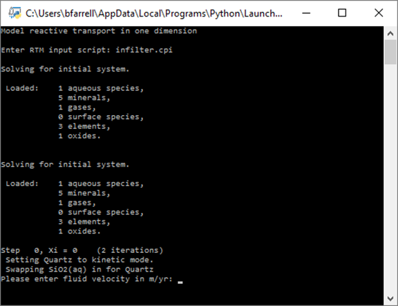
Specify a value of 100 m yr⁻¹ and hit Enter.

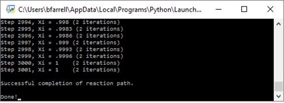
The client will begin time marching, solving the transport and chemical reaction equations at each step of the calculation, and writing banner-style output to the console.

Once the simulation is complete, double-click the “RTM.txt” file to see the results. The file shows the equilibrium state of the inlet fluid, the initial state of each ChemPlugin instance making up the domain, and those same ChemPlugin instances after 2, 4, 6, 8, and 10 years of reaction.

The plot below shows the concentration of dissolved silica as a function of position along the aquifer, at the end of the simulation.

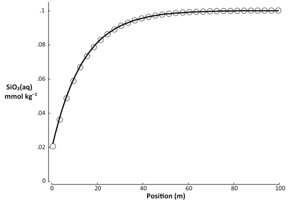
The circles represent the result of modeling the same scenario with program X1t.

---

Authors

Craig M. Bethke and Brian Farrell. © Copyright 2016–2024 Aqueous Solutions LLC. This lesson may be reproduced and modified freely to support any licensed use of The Geochemist's Workbench® software, provided that any derived materials acknowledge original authorship.

References

Bethke, C.M., 2022, Geochemical and Biogeochemical Reaction Modeling, 3^rd ed. Cambridge University Press, New York, 520 pp.

Bethke, C.M., 2024, The Geochemist's Workbench®, Release 17: ChemPlugin™ User's Guide. Aqueous Solutions LLC, Champaign, IL, 303 pp.

---