Direct output

Direct Output is part of a free web series, ChemPlugin Modeling with Python, by Aqueous Solutions LLC.

On-demand Output

Although the “Report()” function is perhaps the most common mode of rendering the results, the client can also prompt a ChemPlugin instance to write out results directly, either as a print-format or plot-format dataset. Direct output provides a method for communicating results to the software user with a minimum of effort on the part of the client.

A client program can trigger output to a print-format dataset using the “PrintOutput()” member function. The function triggers an instance to write a data block representing the instance's current state to a human-readable text file.

    cp.PrintOutput("myPrint.txt")
    cp.PrintOutput() # to same dataset
                

When passed a file name the instance appends a data block to that file, if it is open for output, or opens and writes to a new file of that name. Calling the function without an argument causes the block to be appended to whatever dataset is currently open.

An optional second argument causes the instance to post an identifying label at the head of the data block being written.

    cp.PrintOutput("myPrint.txt", "Tank 3")
    cp.PrintOutput("", "Initial") # same dataset
                

As an example, if we were to add two calls to “PrintOutput()” to the time marching loop below

    # Initialize the instance
    cp.Initialize()
    cp.PrintOutput("myPrint.txt")
    
    # Time Marching loop
    while True:
        deltat = cp.ReportTimeStep()
        if cp.AdvanceTimeStep(deltat): break
        if cp.AdvanceChemical(): break
        cp.PrintOutput()
                

the program would write into “myPrint.txt” a block representing the initial condition, followed by blocks representing the result after completing each time step.

In a second example

    # Initialize the instance
    cp.Initialize()
    cp.PrintOutput("Initial.txt")
    
    # Time Marching loop
    while True:
        deltat = cp.ReportTimeStep()
        if cp.AdvanceTimeStep(deltat): break
        if cp.AdvanceChemical(): break
        cp.PrintOutput("Path.txt")
                

the initial condition would be written to “Initial.txt” and results of the time stepping to “Path.txt”.

Plot format datasets are meant to be read by the Gtplot program supplied with the GWB. Plot-format datasets provide for a simple method for graphically rendering the results of a ChemPlugin simulation for an individual instance.

A plot-format dataset consists of three parts: a header, a series of data blocks, and a trailer. All three are needed if Gtplot is to render the data graphically.

    cp.PlotHeader("myPlot.gtp")
    cp.PlotBlock() # repeat as desired
    cp.PlotTrailer()
                

To create a plot dataset, a client calls “PlotHeader()” once and “PlotBlock()” each time it wants to add the results for a time step. When function “ReportTimeStep()” detects the end of a simulation, it automatically appends the dataset trailer. For this reason, it is commonly not necessary to call “PlotTrailer()”, although doing so simply overwrites any existing trailer and hence is harmless.

As an example, the time marching loop

    # Initialize the instance
    cp.Initialize()
    cp.PlotHeader("myPlot.gtp")
    cp.PlotBlock()
    
    # Time Marching loop
    while True:
        deltat = cp.ReportTimeStep()
        if cp.AdvanceTimeStep(deltat): break
        if cp.AdvanceChemical(): break
        cp.PlotBlock()
        
    cp.PlotTrailer() # Not needed
                

creates a valid plot-format dataset “myPlot.gtp” that contains the initial condition and the instance's state after each step in the time marching loop.

Task 1: Creating print and plot output datasets

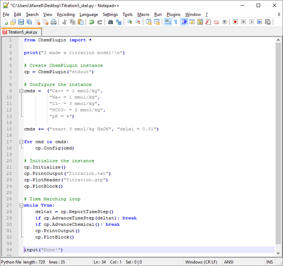
Working again with a variation of our simple titration model, let's set up the client to produce a human-readable printout and a plot output dataset that can be viewed in Gtplot. Open Titration5_skel.py in Notepad++.

Where the instance is initialized, replace the three lines beginning “# >>>” with code to open and write new output files with information about the initial chemical state. Name the print-format dataset “Titration.txt” and the plot-format dataset “Titration.gtp”.

    # Initialize the instance
    cp.Initialize()
    # >>> Write print output to "Titration.txt" <<<
    # >>> Write a header to "Titration.gtp" <<<
    # >>> Append a data block to "Titration"gtp <<<
                

    cp.PrintOutput("Titration.txt")
    cp.PlotHeader("Titration.gtp") 
    cp.PlotBlock()
                    

Within the time marching loop, replace the three lines beginning “# >>>” with code to append blocks of results after each time step to the two files we've created.

    # Time Marching loop
    while True:
        deltat = cp.ReportTimeStep()
        if cp.AdvanceTimeStep(deltat): break
        if cp.AdvanceChemical(): break
        # >>> Append a print block <<<
        # >>> Append a plot block <<<
        
    # >>> Do we need a trailer? <<<
                

        cp.PrintOutput()
        cp.PlotBlock()
                    

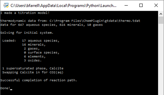
Save your script and rerun. The Command Prompt should look like this:

We see the print statement, some limited console output as a result of using the "stdout" argument in the constructor, and the input statement here, but the bulk of our results have been written to separate datasets.

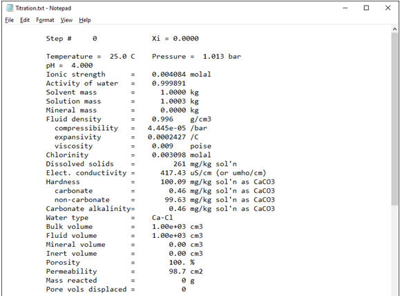
Look in your working directory for the print output dataset “Titration.txt” and double-click to open it.

The first block of data shows the chemical state at Xi = 0, the initial system. The first part of the block shows a variety of chemical and physical properties of the fluid, such as pH, ionic strength, and density:

Next, any reactants are listed, including the amount left to be added at the current point in the simulation and the total amount added so far.

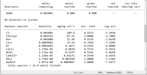
The following sections display the concentration of species in solution, the saturation state of minerals, gas fugacity, and the composition of the system in terms of thermodynamic components and elements.

Subsequent blocks repeat the information discussed above at each increment in reaction progress, Xi.

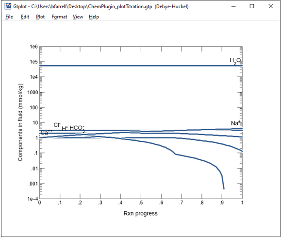
Now go to the working directory and double-click on the Titration.gtp file to launch Gtplot.

Double click on the x axis label and for “Variable type” choose “Reactant properties”, then choose the variable “Mass reacted, NaOH” and select “mmol” for the units.

On the Y Axis pane choose “Chemical parameters” and select pH.

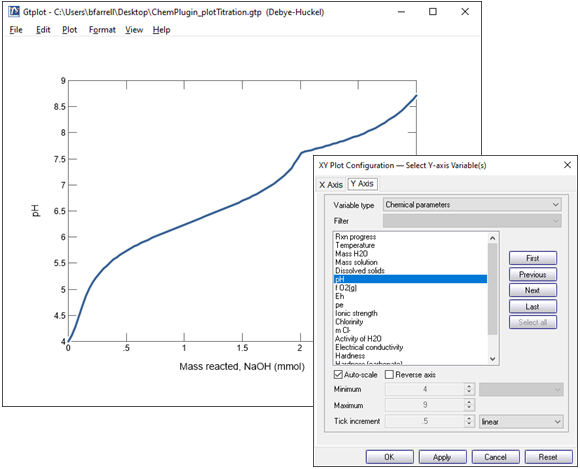
The pH increases from its initial value of 4, as we saw earlier on the command prompt. The pH clearly does not vary linearly with reacted NaOH, however. On the contrary, it changes quickly early on in the simulation, then slowly later on. After about 2 mmoles of NaOH is added, the pH response to the base addition abruptly changes.

Change the y axis variable type to “Minerals” and select Calcite.

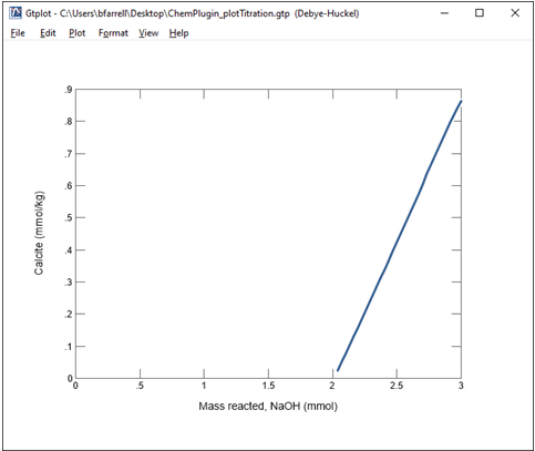
We see here that the onset of calcite precipitation corresponds to the irregularity observed in the previous plot.

Finally, change the y axis variable type to “Species concentration”, and for Filter, select “HCO3-“, then hit the “Select all” button.

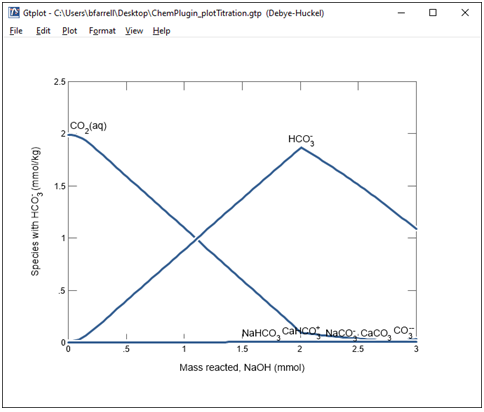
As we saw earlier, CO₂(aq) is the predominant carbon species at low pH. As the pH increases, however, it is converted primarily to the HCO₃^- ion, as well as several other species. The total amount of dissolved carbon decreases at the end of the simulation due to the calcite precipitation.

Self-scheduled Output

As a third option for retrieving calculation results, a client can use the “Config()” member function to turn on print output, plot output, or both. Optionally, the client may call “Config()” to set variables controlling the frequency of output.

A client turns on self-scheduled output to a print-format dataset with the “print” configuration command

    cp.Config("dxprint = 0.1")
        or
    cp.Config("print = on")
        or
    cp.Config("print = off")  
                

and sets the interval between output points with the “dxprint” configuration command.

A client turns on self-scheduled output to the plot dataset with the “plot” command

    cp.Config("dxplot = 0.001")
        or
    cp.Config("dxplot = 0") # each step
        or
    cp.Config("plot = on")  
        or
    cp.Config("plot = off")  
                

and sets the minimum spacing in reaction progress between plot output points with the “dxplot” configuration command.

Task 2: Self-scheduling datasets

Returning to our script in Notepad++, delete all calls to the member functions controlling on-demand output: “PrintOutput()”, “PlotHeader()”, “PlotBlock()”, and “PlotTrailer()”.

Find where the configuration commands are entered and add one more line to the list of commands:

    cmds += ("print = on", "plot = on")
                

Remember, the += operator is used to add additional items (in this case, the new configuration commands) to the cmds list. The “Config()” member function passes those configuration commands in the list to the ChemPlugin instance.

By simply including the additional configuration commands, ChemPlugin is prompted to create print-format and plot-format datasets and writes output at regular intervals.

Save your script and rerun. As before, the Command Prompt should look like this:

Look in your working directory for the new output files produced automatically by the ChemPlugin instance. They are named “ChemPlugin_output.txt” and “ChemPlugin_plot.gtp” by default, but you can use the configuration command “suffix” to append a string to the file name. For example,

    cmds += ("print = on", "plot = on", "suffix = _Titration")
                

produces files named “ChemPlugin_output_Titration.txt” and “ChemPlugin_plot_Titration.gtp”.

Authors

Craig M. Bethke and Brian Farrell. © Copyright 2016–2024 Aqueous Solutions LLC. This lesson may be reproduced and modified freely to support any licensed use of The Geochemist's Workbench® software, provided that any derived materials acknowledge original authorship.

References

Bethke, C.M., 2022, Geochemical and Biogeochemical Reaction Modeling, 3^rd ed. Cambridge University Press, New York, 520 pp.

Bethke, C.M., 2024, The Geochemist's Workbench®, Release 17: ChemPlugin™ User's Guide. Aqueous Solutions LLC, Champaign, IL, 303 pp.