
Acid drainage
Acid Drainage is part of a free web series, GWB Online Academy, by Aqueous Solutions LLC.
What you need:
- GWB Standard recommended
-
Input files:
 AcidDrainage.rea, Co-Precipitation.rea
Download this unit to use in your courses:
- Lesson plan (.pdf)
- PowerPoint slides (.pptx)
Click on a file or right-click and select “Save link as…” to download.
Introduction
Acid drainage is a persistent environmental problem in many mineralized areas. The problem is especially pronounced in areas that host or have hosted mining activity (e.g., Lind and Hem, 1993), but it also occurs naturally in unmined areas. The acid drainage results from weathering of sulfide minerals which produce hydrogen ions and contribute dissolved metals to solution (e.g. Blowes et al., 2005).
Not all drainage, however, is acidic or rich in dissolved metals (e.g., Ficklin et al., 1992; Mayo et al., 1992, Plumlee et al., 1992). Drainage from mining districts in the Colorado Mineral Belt ranges in pH from 1.7 to greater than 8 and contains total metal concentrations ranging from as low as about 0.1 mg kg−1 to more than 1000 mg kg−1. The primary controls on drainage pH and metal content seem to be (1) the exposure of sulfide minerals to weathering, (2) the availability of atmospheric oxygen, and (3) the ability of nonsulfide minerals to buffer acidity.
In this lesson we construct geochemical models to consider how the availability of oxygen and the buffering of host rocks affect the pH and composition of acid drainage.
Task 1: Role of atmospheric oxygen
To investigate how the presence of atmospheric oxygen affects the reaction of pyrite (FeS2) with oxidizing groundwater, we construct a simple model in React. Double-click on file “AcidDrainage.rea”, and when React opens, look at the Basis pane
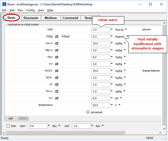
The Basis pane describes a hypothetical groundwater at 25°C that has equilibrated with atmospheric oxygen but is no longer in contact with it.
Now move to the Reactants pane
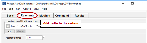
We add pyrite to the system, letting it react to equilibrium with the fluid.
On the Config → Suppress… dialog
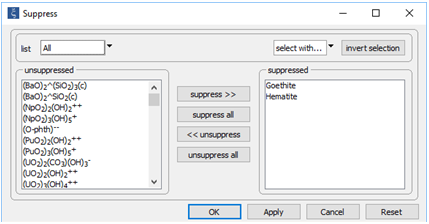
we've suppressed hematite (Fe2O3), which does not form directly at low temperature, and goethite (FeOOH); each of these minerals is more stable thermodynamically than the ferric precipitate observed to form in acid drainage.
Finally, on Config → Output…, the suffix “_isolated” will be applied to datasets produced by the run

Trace the simulation by selecting Run → Go.
Use Gtplot to plot pH of the fluid versus pyrite reacted. Plot as well the concentration of the dissolved oxygen species versus pyrite reacted. How much pyrite dissolves before the reaction ceases? What appears to limit further dissolution?
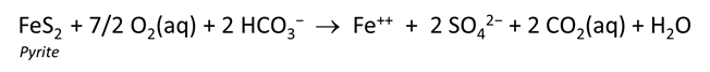
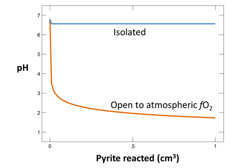
The fluid's pH changes slightly, decreasing from 6.8 to about 6.6
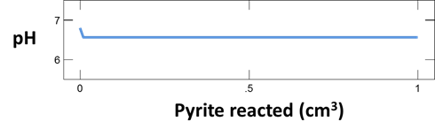
The reaction proceeds until the O2(aq) has been consumed, dissolving a small amount of pyrite according to
To see how contact with atmospheric oxygen might affect the reaction, we repeat the calculation, assuming this time that oxygen fugacity is fixed at its atmospheric level. To do so, return to the Reactants pane and click  → Fixed → Gas… → O2(g)
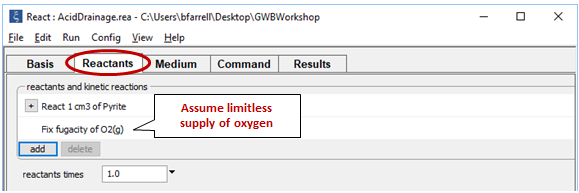
In this case, the reaction will proceed without exhausting the oxygen supply, which in the calculation is limitless.
On Config → Output…, change the suffix to “_atmospheric”

Rerun the simulation by selecting Run → Go. How does contact with the atmosphere affect the resulting drainage chemistry? What iron and sulfur species are particularly important?
The results of the open-system model are shown in orange, together with the previous calculation in blue. Reaction proceeds without exhausting the oxygen supply, which is limitless, driving pH to a value of about 1.7
Initially, pyrite oxidation in the model proceeds according to the reaction
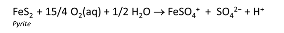
as shown below, producing H+ and thus driving the fluid acidic. According to the model, the pyrite dissolution produces ferric iron in an ion pair with sulfate
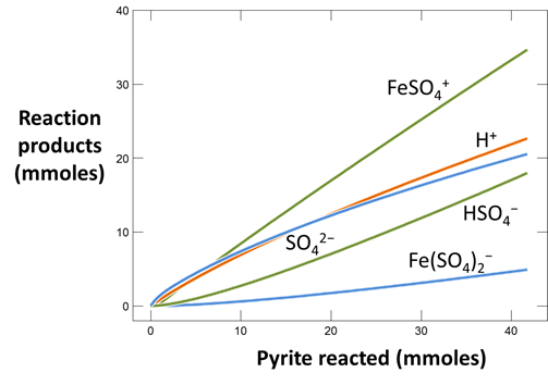
As the pH decreases, bisulfate comes to dominate sulfate and a second reaction

becomes important. This reaction produces no free hydrogen ions and hence does not contribute to the fluid's acidity.
Task 2: Buffering by wall rocks
The most important control on the chemistry of drainage from mineralized areas (once we assume access of oxygen to the sulfide minerals) is the nature of the nonsulfide minerals available to react with the drainage before it discharges to the surface (e.g., Sherlock et al., 1995). These minerals include gangue minerals in the ore, the minerals making up the country rock, and the minerals found in mine dumps. The drainage chemistry of areas in which these minerals have the ability to neutralize acid differs sharply from that of areas in which they do not.
To model the effect of carbonate minerals on drainage chemistry, we continue our calculations from the previous task (in which we reacted pyrite with a hypothetical groundwater in contact with atmospheric oxygen).
Return to the Basis pane and include calcite (CaCO3) in the initial system. To do so, click on the swap button  next to the basis entry for “HCO3−” and select Mineral… → “Calcite”. Change the units to “cm3” and set a value of "10". Finally, click the pulldown to the right of the units for Ca++ and select “Balance species”
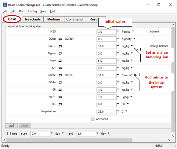
The setting sets the fluid to be in equilibrium with 10 cm3 of the carbonate mineral calcite.
On Config → Output…, set the suffix “_calcite”
Trace the simulation by selecting Run → Go.
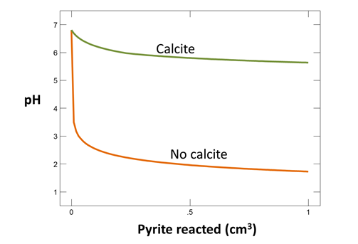
How does the resulting pH differ from the previous calculation in which the fluid remained open to exchange with atmospheric O2, but no calcite was present to react with the drainage? How do the resulting drainage chemistries differ?
Now take a look at the minerals that are consumed or precipitated in the simulation as pyrite dissolves. How much calcite is consumed per cm3 of pyrite reacted?
In contrast to the previous calculation (plotted in orange), the fluid maintains a near-neutral pH, reflecting the acid-buffering capacity of the calcite
As the pyrite dissolves by oxidation, calcite is consumed and ferric hydroxide precipitates. Calcium and sulfate accumulate in the fluid, eventually causing gypsum to saturate and precipitate
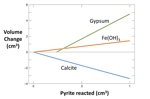
In the calculation, reaction of 1 cm3 of pyrite consumes about 3.4 cm3 of calcite, demonstrating that considerable quantities of buffering minerals may be required in mineralized areas to neutralize drainage waters.
In the two calculations (one including, the other excluding calcite), the resulting fluids differ considerably in composition. After reaction of 1 cm3 of pyrite at atmospheric oxygen fugacity, the compositions are
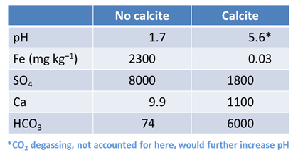
Whereas pyrite oxidation in the absence of calcite produces H-Fe-SO4 drainage, the reaction in the presence of calcite yields a Ca-HCO3-SO4 drainage.
Task 3: Co-Precipitation
As pH rises, the metals content of drainage waters tends to decrease. Some metals, like iron and aluminum, precipitate directly from solution to form oxide, hydroxide, and oxy-hydroxide phases. They initially form colloidal and suspended phases known as hydrous ferric oxide (HFO) or hydrous aluminum oxide (HAO), both of which are highly soluble under acidic conditions but nearly insoluble at near-neutral pH.
The concentrations of other metals attenuate when the metals sorb onto the surfaces of precipitating minerals. HFO, for example, has a large specific surface area and is capable of sorbing metals from solution in considerable amounts. The process by which minerals form and then adsorb metals from solution is known as co-precipitation.
Let's construct a model in which reaction of a hypothetical drainage water with calcite leads to the precipitation of ferric hydroxide [Fe(OH)3, which we use to represent HFO] and the sorption of dissolved species onto this phase. To start, double-click on file “coprecipitation.rea”.
On the Config → Redox Couples… dialog
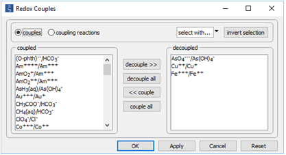
we've prepared the calculation by disenabling the redox couple between trivalent and pentavalent arsenic (arsenite and arsenate, respectively). As well, we disenable the couples for ferric iron and cupric copper, since we will not consider either ferrous or cuprous species.
Moving to the Basis pane
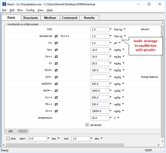
we define an initial fluid representing the unreacted drainage. We set the fluid's iron content by assuming equilibrium with jarosite [NaFe3(SO4)2(OH)6] and prescribe a high content of dissolved arsenite, arsenate, cupric copper, lead, and zinc.
On the Reactants pane
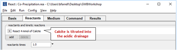
we titrate 4 mmoles of calcite into the initially acidic drainage.
Opening Config → Sorbing Surfaces…, we see we've read in the “FeOH+.sdat” dataset
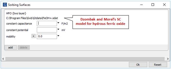
This is Dzombak and Morel's (1990) compilation of surface complexation reactions for hydrous ferric oxide, which will precipitate in our simulation. We assume that the precipitate remains suspended in solution with its surface in equilibrium with the changing fluid chemistry.
Going to Config → Stepping…
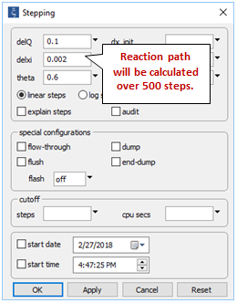
we prescribe a smaller step size than the default value used by React.
On the Config → Suppress… dialog
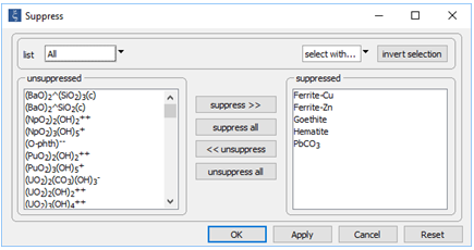
we've suppressed hematite and goethite, (both of which are more stable than ferric hydroxide) two ferrite minerals (e.g., ZnFe2O4), which we consider unlikely to form, and the PbCO3 ion pair, the stability of which in the database is almost certainly erroneous.
Finally, on Config → Output…, the suffix “_coprecipitation” will be applied to datasets produced by the run

Trace the simulation by selecting Run → Go.
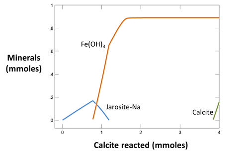
Use Gtplot to make a graph showing the minerals formed as calcite is reacted into the drainage. Plot as well the “fraction sorbed” of the various metals as a function of the pH, which increases during the course of the simulation.
In the calculation, calcite dissolves into the drainage according to

and

consuming H+ and causing pH to increase. The shift in pH drives the ferric iron in solution to precipitate as ferric hydroxide, according to

A total of about 0.89 mmol of precipitate forms over the reaction path
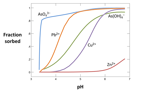
The distribution of metals between solution and the ferric hydroxide surface varies strongly with pH, which increases as the water reacts with calcite
Is is useful to compare the capacity for each metal to be sorbed (the amount of each that could sorb if it occupied every surface site) with the metal concentrations in solution. How might we do this?
To calculate the capacities, we take into account the amount of ferric precipitate formed in the calculation (0.89 mmol), the number of moles of strongly and weakly binding surface sites per mole of precipitate (0.005 and 0.2, respectively, according to the surface complexation model) and the site types that accept each metal [arsenate and arsenite sorb on weak sites only, whereas lead, copper, and zinc sorb on both strong and weak].
Comparing the initial metal concentrations to the resulting capacities for sorption
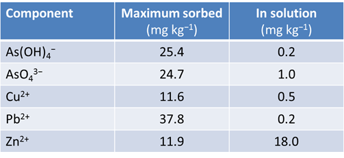
we see that the precipitate forms in sufficient quantity to sorb the arsenic initially present as well as the lead and copper, but only a fraction of the zinc. An initial consideration in evaluating the ability of co-precipitation to attenuate metal concentrations, therefore, is whether the sorbing mineral forms in a quantitiy sufficient to sorb the water's metal content.
Authors
Craig M. Bethke and Brian Farrell. © Copyright 2016–2026 Aqueous Solutions LLC. This lesson may be reproduced and modified freely to support any licensed use of The Geochemist's Workbench® software, provided that any derived materials acknowledge original authorship.
References
Bethke, C.M., 2022, Geochemical and Biogeochemical Reaction Modeling, 3rd ed. Cambridge University Press, New York, 520 pp.
Bethke, C.M., B. Farrell, and M. Sharifi, 2026, The Geochemist's Workbench®, Release 18: GWB Reaction Modeling Guide. Aqueous Solutions LLC, Champaign, IL, 219 pp.
Blowes, D.W., C.J. Ptacek, J.L. Jambor and C.G. Weisener, 2005, The Geochemistry of Acid Mine Drainage. In B.S. Lollar (ed.), Environmental Geochemistry, Elsevier, Amsterdam, 149–204.
Lind, C.J. and J.D. Hem, 1993, Manganese minerals and associated fine particulates in the streambed of Pinal Creek, Arizona, U.S.A., a mining-related acid drainage problem. Applied Geochemistry 8, 67–80.
Sherlock, E.J., R.W. Lawrence and R. Poulin, 1995, On the neutralization of acid rock drainage by carbonate and silicate minerals. Environmental Geology 25, 43–54.
Comfortable with acid drainage?
Move on to the next topic, Waste Injection Wells, or return to the GWB Online Academy home.