Surface complexation

Jump to:

Introduction Task 1: Groundwater chromatography Task 2: Two dimensions Animation of two-dimensional example Authors and references

Surface Complexation is part of a free web series, GWB Online Academy, by Aqueous Solutions LLC.

What you need:

GWB 2023 Professional recommended
Input files: 3metals.x1t, 3Metals.x2t

Download this unit to use in your courses:

Lesson plan (.pdf)
PowerPoint slides (.pptx)

Click on a file or right-click and select “Save link as…” to download.

Introduction

We begin our discussion of surface complexation with Irving Langmuir's work, which greatly improves upon the K_d and Freundlich isotherms. In the Langmuir model, a species sorbs and desorbs according to a reaction such as:

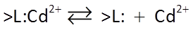
where >L:Cd²⁺ is a sorbing site occupied by a cadmium ion, and >L: is an unoccupied site.

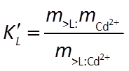
The Langmuir reaction has an equilibrium constant K and a mass action equation:

It additionally maintains a mass balance on the sorbing sites. The model, for this reason, does not predict that species can sorb indefinitely, since the number of sites available is limited

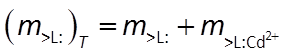
Combining the mass action and mass balance equations results in the Langmuir equation:

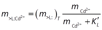
Where the concentration of Cd²⁺ is much smaller than K, the sorbed concentration varies in proportion to the concentration of the dissolved species. As the dissolved concentration increases to values greater than K, in contrast, the sorbed concentration approaches the concentration of sorbing sites, as shown below:

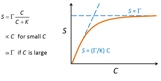
The Langmuir equation behaves very much like the Michaelis-Menten and Monod equations, described in the Biodegradation and Microbial Populations sections, respectively.

Experiments with natural sediments reveal a Freundlich-like nature to their isotherms, although the approach is purely empirical. A mechanistically based Langmuir model with multiple sorbing sites can reproduce this observation.

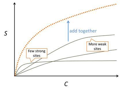
We consider a surface complexation model to be a multisite competitive Langmuir model that accounts for site protonation and deprotonation as well as electrostatic forces.

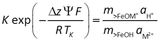
In order for an ion to sorb from solution, it must first move through an electrical potential field and then react chemically at the surface. Moving a positively charged ion toward a positively charged surface, for example, requires that work be done on the ion, increasing the system's free energy. An ion of the same charge escaping the surface would have the opposite energetic effect.

An equilibrium constant K represents the chemical effects of free energy. Multiplying K by the Boltzman factor (shown below) gives a complete account of the reaction's free energy.

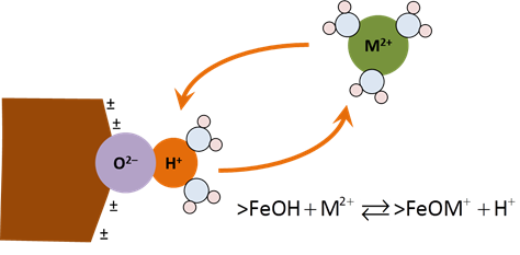
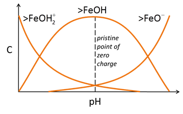
Three main classes of reactions are involved in surface complexation models. Each site can protonate or deprotonate to form surface species such as >FeOH₂⁺ or >FeO⁻. In the absence of any complexing ions, the figure below explains the nature of surface sites and surface charge as a function of pH

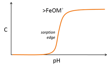
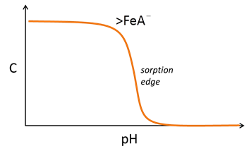
The sites can react with cations and anions from solution to form complexes, such as >FeOM⁺ or >FeA⁻. Increasing pH causes sites to deprotonate and complex with bivalent cations

Anion complexation, conversely, is typically favored at low pH

In this example, we'll use the compilation of surface complexation reactions from Dzombak and Morel (1990). They studied sorption onto hydrous ferric oxide (HFO = FeOOH · nH₂O). Looking at the dataset, the sorbing sites are just like basis species in a thermo dataset. The two types of sites, strong and weak, give a Freundlich-like character to isotherms

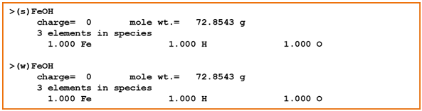
Sorbing minerals can be associated with one or more sorbing sites. We use the mineral Fe(OH)₃(ppd) as a proxy for HFO. According to the model, there are forty times more weak sites than strong sites

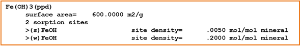
The strong sites can protonate, deprotonate, or complex cations. The weak sites can additionally complex anions

Task 1: Groundwater chromatography

Three heavy metal contaminants—Hg²⁺, Pb²⁺, Zn²⁺—pass into an aquifer in equal concentration. Sediment grains in the aquifer are coated with small amounts of hydrous ferric oxide, HFO or “rust”, onto which the contaminants can complex.

We'd like to construct a reactive transport model to show how the contaminants behave as they migrate with the flowing groundwater, accounting for the surface complexation.

To start, double-click on file “3metals.x1t”. The configuration is much like the simulation we've been tracing (“Pulse.x1t”), with the addition of two new contaminants and the HFO coatings.

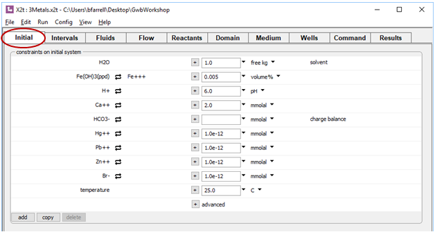
Moving to the Initial pane

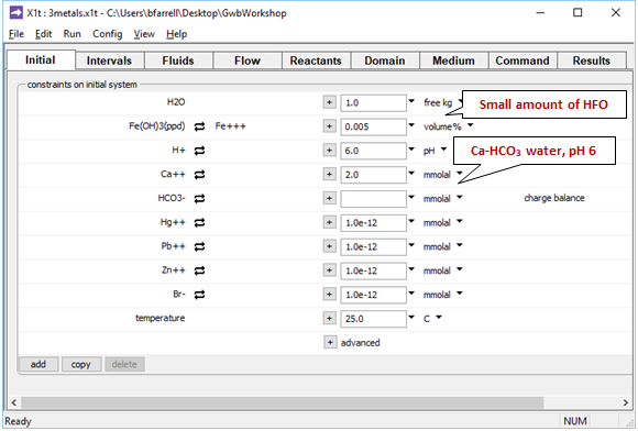
we see the aquifer contains a small amount of Fe(OH)₃ precipitate, a proxy for HFO. The pore fluid is a Ca-HCO₃ water, which provides a buffer in the simulation.

On the Fluids pane

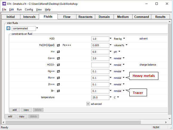
fluid passing into the domain contains 0.1 mmolal Hg²⁺ and Zn²⁺ contaminants, in addition to Pb²⁺. We've set the same concentration for Br⁻, which serves in the calculation as a tracer, since it neither reacts nor sorbs to HFO.

Opening Config → Sorbing Surfaces…, we see we've read in the “FeOH+.sdat” dataset

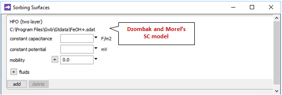
containing Dzombak and Morel's (1990) compilation of surface complexation reactions.

On the Config → Redox Couples… dialog

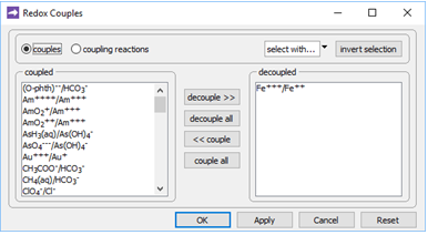
we see that redox coupling between ferric and ferrous iron has been disabled. This setting explains why we've been able to include Fe³⁺ species and minerals in the simulation, without setting basis entries representing Fe²⁺ or redox state.

Going to Config → Options…

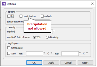
the “precipitation” option has been deselected. This setting prevents stable but slow-forming ferric minerals like goethite (FeOOH) from appearing in the simulation, at the expense of the Fe(OH)₃ precipitate.

On the Config → Suppress… dialog

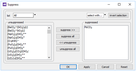
we've suppressed the PbCO₃ ion pair, the stability of which in the database is almost certainly erroneous.

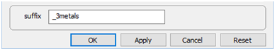
Finally, on Config → Output…, the suffix “_3metals” will be applied to datasets produced by the run

Trace the simulation by selecting Run → Go.

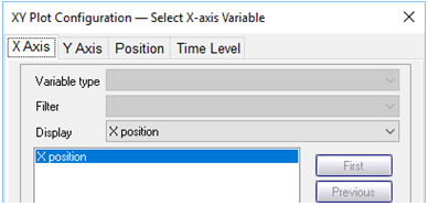
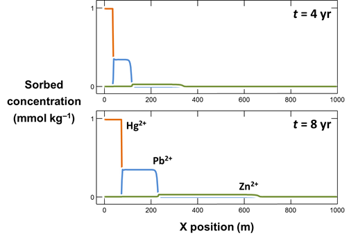
Use Xtplot to make a graph showing how the concentrations of the Hg²⁺, Pb²⁺, Zn²⁺, and Br⁻ components vary along the aquifer, after 4 years and 8 years of reaction. Hint: double-click on the x-axis label and for “Display” choose “X position”

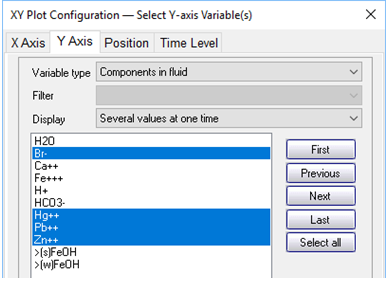
On the Y Axis pane choose “Components in fluid” and select Br⁻, Hg²⁺, and so on, with a linear axis. If it is not already selected, choose “Several values at one time” for “Display”

Why do Hg²⁺, Pb²⁺, Zn²⁺, and Br⁻ migrate along the aquifer at different rates? Why at some points in the aquifer are Pb²⁺ and Zn²⁺ concentrations predicted to be greater than in the inlet fluid?

Make a second plot like the first, but showing the concentrations of sorbed Hg²⁺, Pb²⁺, and Zn²⁺ along the aquifer (Y Axis, “Components in sorbate”). Why do the contaminants segregate into zones as they sorb?

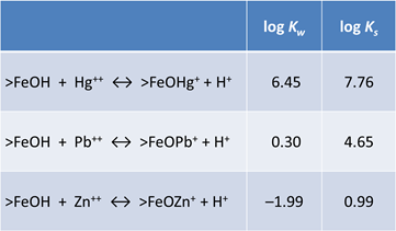
From the binding constants, we see that Hg⁺⁺ binds more strongly to HFO than Pb⁺⁺, which in turn binds more strongly than Zn⁺⁺

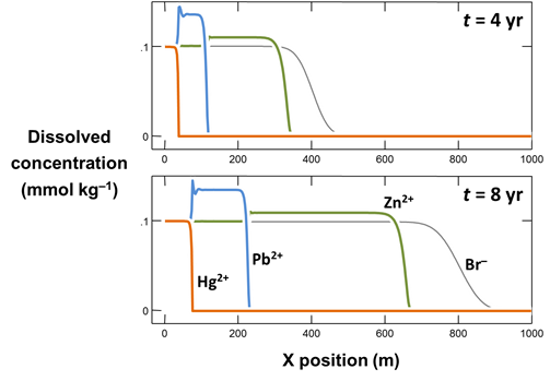
The figure below shows the concentrations of metal ions in the groundwater after 4 and 8 years of transport. As the contaminated fluid in the simulation passes into the aquifer, the metals separate due to differential sorption. The Hg²⁺, which sorbs most strongly, is retarded the most, while the weakly sorbing Zn²⁺ ion is least retarded

In the plot of sorbed metal concentrations, below, the Hg²⁺ ions, which sorb to the ferric surface most strongly, exclude the other metals. Once Hg²⁺ is exhausted from the fluid, the Pb²⁺begins to sorb, and the Zn²⁺ sorbs where the Pb²⁺ is depleted, leaving each metal bound within its own chromatographic band

Where Hg²⁺ in the migrating fluid passes from the first to the second band, it displaces Pb²⁺ from the sorbate, since both metals compete for the same sites. Because there are two sources of dissolved Pb²⁺, the Pb²⁺ concentration rises well above that of the unreacted fluid. At the interface between the second and third bands, similarly, Pb²⁺ displaces Zn²⁺.

As these reactions proceed, the interfaces between the bands migrate slowly downstream, as do the pulses of highest Pb²⁺ and Zn²⁺ concentration.

Task 2: Two dimensions

Let's try a more complex model. Three tanks leak Hg²⁺, Pb²⁺, and Zn²⁺ into an aquifer, where they are entrained by flow along the hydraulic grade.

After 10 years, the sources are controlled and a remediation well is installed down-gradient of the tanks to draw out contaminated groundwater. The remediation well is pumped in the simulation for 40 years.

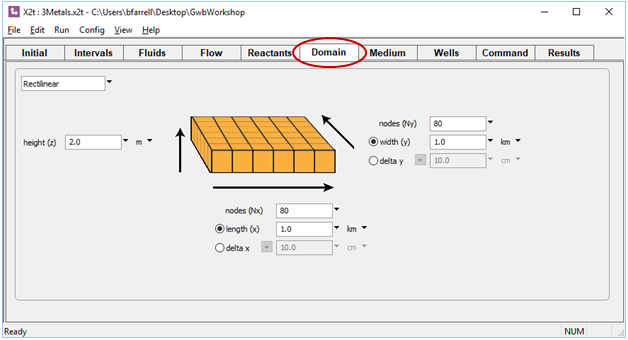
Start X2t by double-clicking on file “3metals.x2t”. On the Domain pane, we see the domain is 1 square km, divided into 6400 nodal blocks

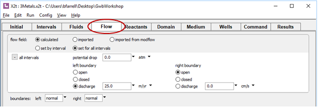
On the Flow pane, we see the background discharge is 25 m yr⁻¹, left to right

The Initial pane specifies a clean fluid

Four wells are defined on the Wells pane. Click to expand any of the entries

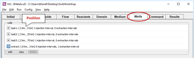
The first three slowly leak the “contamination” fluid into the aquifer over the first 10 years. The remaining well, at the bottom of the list, is the remediation well. It withdraws water from the aquifer, so the injection rate is set to a negative value

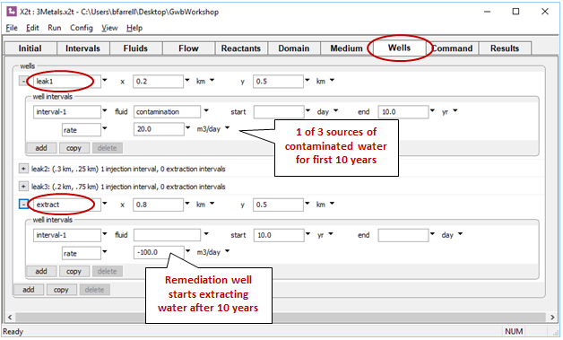
Fluid is withdrawn from the aquifer in the “extract” well, but none is injected, so no injectate chemistry need be specified.

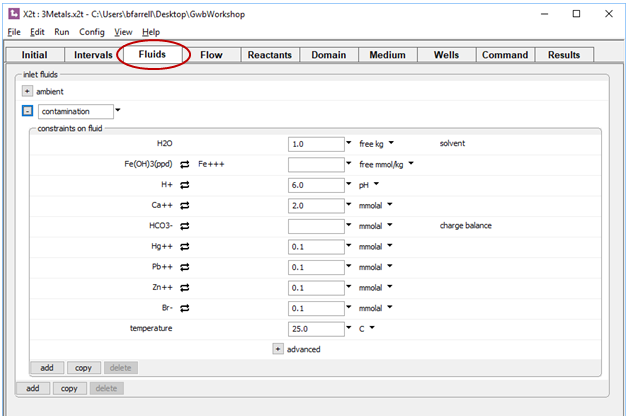
The Fluids pane is where we describe the chemistry of the fluids that will enter the domain over the course of the simulation. The first is a clean fluid, “ambient”, and the second is the comtaminated water that is laden with the inorganic metal pollutants as well as a bromide tracer

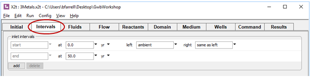
The Intervals pane specifies the duration of the simulation and the fluid crossing the left boundary

You can trace the simulation by selecting Run → Go.

We would like to make animations that show the equipotentials (contours of hydraulic potential) as well as the concentrations of tracer Br or one of the inorganic metal contaminants, Hg²⁺, Pb²⁺, or Zn²⁺.

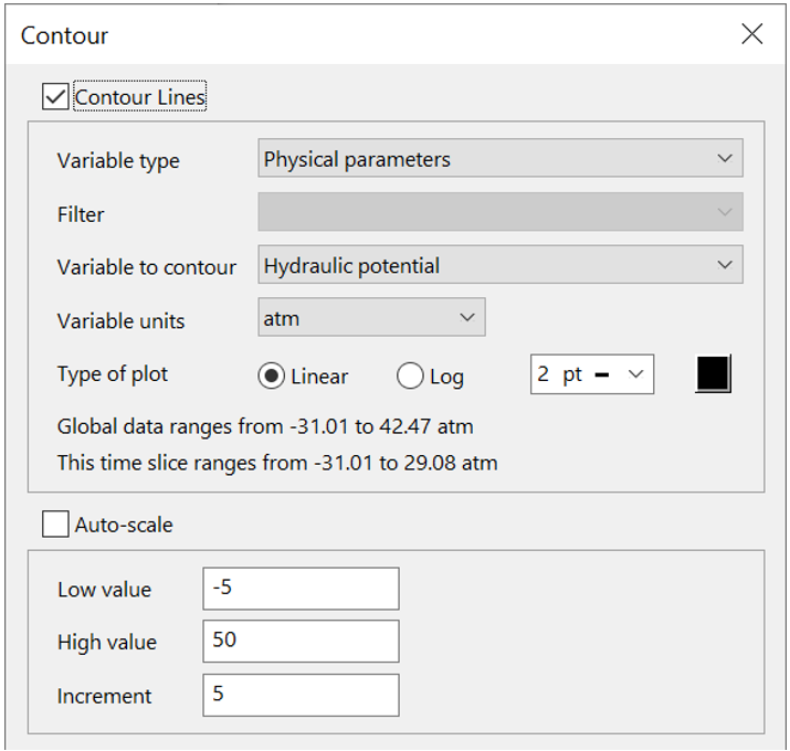
To do so, click to launch Xtplot and go to Plot → Map View. To set up the equipotentials, go to Format → Contour..., choose “Physical parameters”, and select “Hydraulic potential”

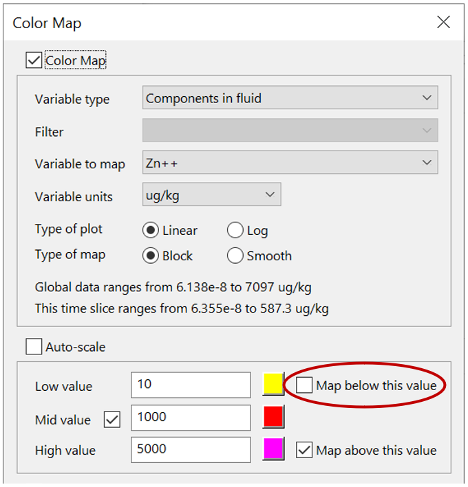
Color map the concentration of the tracer, or one of the metals, from Format → Color Map…, as you did in the previous exercise for sorbing solutes. Remember to select “Components in fluid” and the appropriate basis entry. Remember, you can mask areas of the domain that fall below the low value threshold by unchecking the “Map below this value” check box:

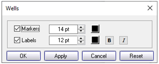
To add markers to your plot showing the well locations, go to Format → Wells…

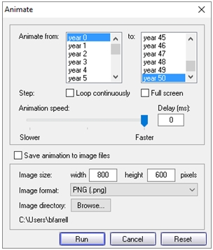
Now, animate your diagrams from the Format → Animate… dialog

From your results, consider the following questions:

How do the injection and production wells affect the flow field in each reaction interval?
Why do Hg²⁺, Pb²⁺, Zn²⁺, and Br⁻ migrate along the aquifer at different rates?
How effective is flushing in removing each of the metals from the aquifer?
Explain how surface complexation reactions can be both beneficial and a hindrance to remediation efforts.

Animation of two-dimensional example

In the simulation, three tanks leak water contaminated with heavy metals into an aquifer for 10 years. At that time, the leaks are controlled and an extraction well begins operation.

Three metals—Hg²⁺, Pb²⁺, and Zn²⁺—sorb in the run according to a surface complexation (two-layer) model, and Br− serves as a non-reactive tracer.

Authors

Craig M. Bethke and Brian Farrell. © Copyright 2016–2024 Aqueous Solutions LLC. This lesson may be reproduced and modified freely to support any licensed use of The Geochemist's Workbench® software, provided that any derived materials acknowledge original authorship.

References

Bethke, C.M., 2022, Geochemical and Biogeochemical Reaction Modeling, 3^rd ed. Cambridge University Press, New York, 520 pp.

Bethke, C.M., B. Farrell, and M. Sharifi, 2024, The Geochemist's Workbench®, Release 17: GWB Reactive Transport Modeling Guide. Aqueous Solutions LLC, Champaign, IL, 191 pp.

Dzombak, D.A. and F.M.M. Morel, 1990, Surface Complexation Modeling. Wiley, New York, 393 pp.

Comfortable with Surface complexation?

Move on to the next topic, Mobile Colloids, or return to the GWB Online Academy home.