
Microbial populations
Microbial Populations is part of a free web series, GWB Online Academy, by Aqueous Solutions LLC.
What you need:
- GWB Professional recommended
-
Input files:
 As_reduction_scatter.gss,
  ArsenateReduction.rea,
 thermo+Lactate.tdat,
  Microbes.x1t,
thermo_microbes.tdat
Microbes.x1t,
thermo_microbes.tdat
Download this unit to use in your courses:
- Lesson plan (.pdf)
- PowerPoint slides (.pptx)
Click on a file or right-click and select “Save link as…” to download.
Introduction
Chemosynthetic microorganisms derive the energy they need to live and grow from chemical species in the environment, reaping the benefits of the redox disequilibrium characteristic of geochemical environments. The microbes catalyze redox reactions, harvesting some of the energy released and storing it as adenosine triphosphate, or ATP, the cell's energy currency.
A respiring microbe captures the energy released when electrons are transferred from a reduced species in the environment to an oxidized species.
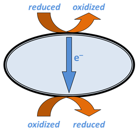
The reduced species, the electron donor, sorbs to a complex of redox enzymes, or a series of such complexes, within the cell membrane. The complex strips from the donor one or more electrons, which cascade through a series of enzymes and coenzymes that make up the electron transport chain to a terminal enzyme complex, also within the cell membrane.
The oxidized species, the electron acceptor, sorbs to the terminal complex and takes up the electrons, becoming reduced. The newly oxidized donating species and the accepting species, now reduced, desorb from the redox complexes and move back into the environment.
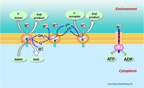
The energy released by the electrons passing through the transport chain does the critical work, driving hydrogen ions from within the cell's cytoplasm across the cell membrane, a process known as proton translocation. The hydrogen ions, under the drive of strong gradients in electrical and chemical potential, reenter the cell through the ATP synthase, a special membrane-bound enzyme. The ATP synthase, activated by movement of the hydrogen ions, binds together adenosine diphosphate (ADP) and orthophosphate ions in the cell's cytoplasm to form ATP.
The Monod equation is the relation most commonly applied to describe the rate at which a microbe metabolizes its substrate. If the electron donor is the limiting reactant, the Monod equation gives reaction rate as
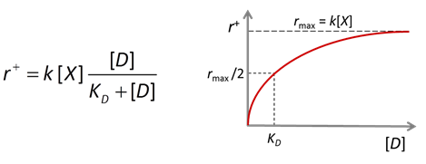
where r+ is the forward reaction rate (mol s−1), k+ is the rate constant (mol mg−1 s−1), [X] is biomass concentration (mg kg−1), D is the concentration of the electron donor, and KD is the half-saturation constant for the donor. If the electron acceptor is limiting, the equation can similarly be written in terms of A, the concentration of the electron acceptor, and KA, the corresponding half-saturation constant for the acceptor. Where substrate concentration is considerably smaller than the half-saturation constant, the reaction rate is proportional to mA. In other words, it is substrate limited. For the opposite case, reaction rate is invariant with respect to substrate concentration.
The Monod equation behaves very much like the Langmuir and Michaelis-Menten equations, described in the Surface Complexation and Biodegradation sections, respectively.
The Monod equation differs from the Michaelis-Menten equation in that it includes as a factor biomass concentration [X], which can change with time
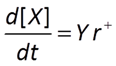
A microbe's growth rate is proportional to its growth yield and the rate of its catabolic (energy yielding) reaction.
The Monod equation predicts the forward rate r+ of reaction, rather than the net rate r, which is the difference r+ − r− between the forward and reverse rates. This distinction is of little practical significance for reactions that liberate significant amounts of free energy, because for those cases the reverse rate is negligible. The aerobic oxidation of organic compounds, for example, is so strongly favored thermodynamically than, in the presence of detectable levels of O2(aq) and the organic substrate, the forward and net rates are indistinguishable.
Metabolisms such as methanogenesis and bacterial sulfate reduction, conversely, liberate sufficiently little energy that in common geochemical environments the forward and reverse rates can be of similar magnitude. In constructing a geochemical model, furthermore, we wish to avoid allowing simulations in which a microbially catalyzed reaction might proceed, impossibly, beyond its point of equilibrium. We should, therefore, account for the effect of thermodynamics on the net rate of reaction.
In considering the energetics of a microbially catalyzed reaction, it is important to recall that progress of the redox reaction is coupled to synthesis of ATP within the cell, so the overall reaction is the redox reaction combined with ATP synthesis. The free energy liberated by the overall reaction is the energy liberated by the redox reaction, less that consumed to make ATP. The overall reaction's equilibrium point is where this difference vanishes; at this point, the forward and reverse rates balance and there is no net reaction.
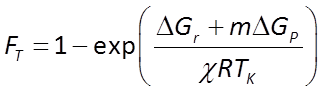
To account for reverse as well as forward reaction, the Monod equation can be modified by appending to it a thermodynamic potential factor, as shown by Jin and Bethke (2005), in which case the equation predicts the net rate of reaction. The thermodynamic factor FT, which can vary from zero to one, is given by
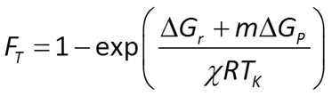
where ΔGr is the free energy change (J mol−1) of the redox reaction, ΔGP is the free energy change (J mol−1) under cellular conditions of the phosphorylation reaction of ADP to produce ATP, m is the number of ATPs produced per reaction turnover, χ is the average stoichiometric number of the overall reaction (number of times the rate determining step, commonly proton translocation, occurs per turnover of the overall reaction), R is the gas constant (8.3143 J mol−1 K−1), and TK is absolute temperature (K). The value of ΔGP under typical physiological conditions is in the range of about 40-50 kJ mol−1.
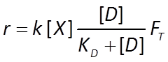
Appending FT to the Monod equation, we write a thermodynamically consistent rate law
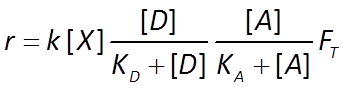
Similarly, the dual Monod equation in thermodynamically consistent form becomes
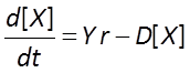
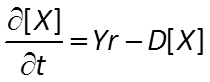
Finally, we allow biomass to decay with time
Task 1: Arsenate reduction by B. arsenicoselenatis
Blum et al. (1998) isolated a bacterial strain Bacillus arsenicoselenatis from muds of Mono Lake, a hypersaline alkaline lake in northern California. Under anaerobic conditions in saline water, over an optimum pH range of 8.5 – 10, the strain can respire using As(V), or arsenate, as the electron acceptor, reducing it to As(III), arsenite.
In a batch experiment, Blum et al. (1998) were able to grow the strain at 20°C on arsenate in saline water, using lactate as the electron donor. The strain oxidized the lactate incompletely to carbonate and acetate, according to the reaction

Capturing energy liberated by the reaction, the microbial population grew almost 40-fold over the course of the experiment, which lasted about 3 days.
Reaction proceeded increasingly rapidly as the microbial population, and hence the system's catalytic ability, increased. After about a day, however, the reaction started to slow, and then it stopped altogether, even though all the lactate and arsenate had yet to be consumed.
In this task, we develop a kinetic description of microbial catalysis and growth observed in the experiment. Following Jin and Bethke (2003), we pay attention to thermodynamic as well as kinetic controls on the reaction rate.
To see Blum et al.'s experimental data, double-click on “As_reduction_scatter.gss”. The GSS file contains measurements of the concentrations of reactant and product species for the microbe's metabolism, as well as the biomass observed at a number of sampling points
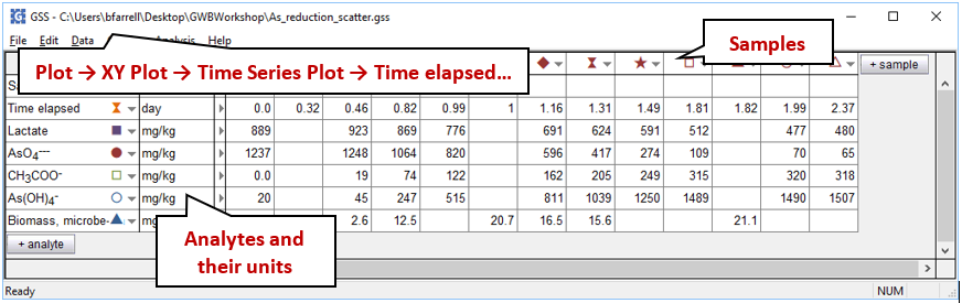
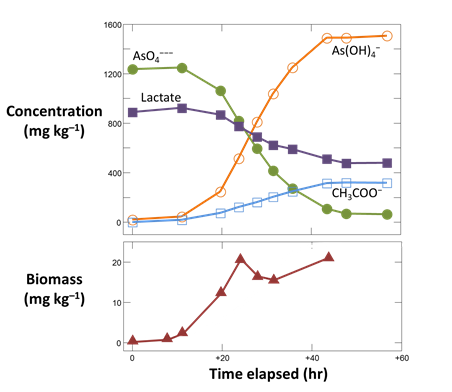
Launch Gtplot by going to Plot → XY Plot → Time Series Plot → Time elapsed…, then plot vs. time the concentrations in the fluid of components As(OH)4 −, AsO4−−−, CH3COO−, and Lactate. In a second graph, plot the growth curve, which is biomass concentration vs. time.
From your results, does reaction continue until all of the lactate and arsenate have been metabolized?
The reaction rate begins to slow around 30 hours, then halts after about 45 hours, even though lactate and arsenate are still available
Now double‐click on “ArsenateReduction.rea” to open a React simulation. Click on File → View → “.\thermo+Lactate.tdat”. This dataset is the “thermo.tdat” compilation we've been using, with an added entry for the lactate ion. Search on “Lactate” to find the redox couple

which has a log K at 20°C, the temperature of the experiment, of 231.4.
On the Config → Redox Couples… dialog
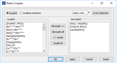
the coupling reactions between arsenite and arsenate, carbonate and acetate, and carbonate and lactate are disabled. Configuring the model in this way provides for the redox disequilibrium that supplies the microbial strain with energy.
On the Basis pane
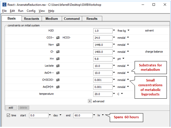
we set the composition of the growth medium, a saline fluid with pH 9.8. We set as well the initial concentrations of lactate and arsenate, and arbitrarily small quantities of the metabolic products acetate and arsenite.
On the Reactants pane
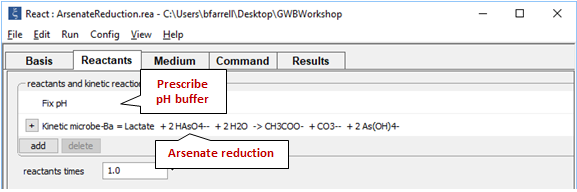
we set a pH buffer and define the microbial rate law, which will take the form
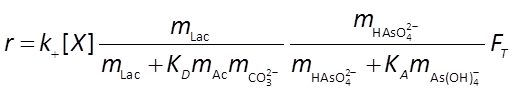
The thermodynamic parameters m, ΔGP, and χ that make up FT
can be estimated from knowledge of the microbe's metabolic pathways, or from energetics. Jin and Bethke (2003) showed that m and χ may be reasonably taken as 2.5 and 4, respectively, and ΔGP is in general about 50 kJ mol−1.
The kinetic parameters k+, KD, KA, on the other hand, need to be inferred from the experimental results. We'll begin with initial guesses to their values, and then refine them by progressively fitting the model results to experimental data.
To do so, we set the values of KD and KA to zero initially, forcing the kinetic factors FD and FA to one, their likely values at the onset of reaction, when lactate and arsenate are abundant, but acetate, carbonate, and arsenite are not.
We further choose an initial value for k+ of 10−9, a reasonable assumption since rate constants for microbially catalyzed reactions tend to fall within a narrow range.
Expanding the block for the microbial reaction, we see those assumptions set out:
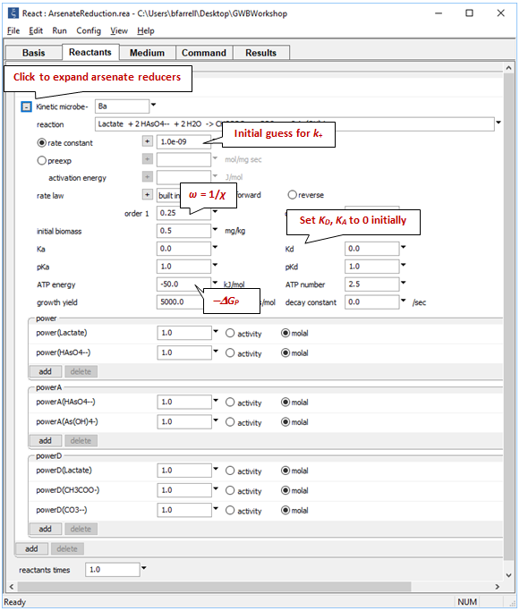
Here we have set the coefficients in the kinetic rate law, the growth yield and decay coefficient, and the initial size of the microbial population. We specify the average stoichiometric number by setting variable ω (“order1”) to 1/ χ. “ATP energy” is −ΔGP (note the negative sign); “ATP number” is m.
Take note of the suffix
and trace the model by selecting Run → Go.
Plot against time the concentrations of the “As(OH)4−”, “AsO4−−−”, “CH3COO−”, and “Lactate” components, in mmolal units.
Superimpose the experimental data stored in the GSS file onto your plot by dragging “As_reduction_scatter.gss” from the course folder into your Gtplot window, then click Yes on the pop-up. Your diagram should look like this
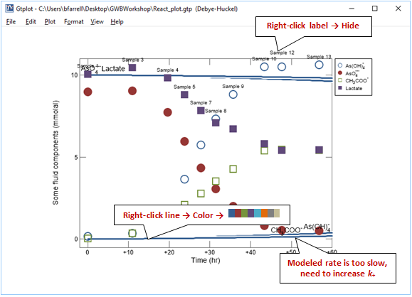
Before continuing, hide the labels for the scatter data and simulation results. Next, match the colors of the simulation results with the experimental data. Right-click one of the dark blue lines corresponding to the model results and choose Color →  . The setting automatically assigns colors to each line using a short color palette. We've chosen the marker colors in GSS to match these colors.
Note: you can also color lines individually. Right-click on a line and choose Color, then uncheck “Use For All Lines”, then set the color of any line as desired.
You'll notice that the lactate and arsenate components are not consumed as quickly in the model as they are in the experiment. To try to improve the fit, increase the rate constant and rerun the simulation. Your plot will update itself when the run completes.
By adjusting k+ and rerunning the model a few times you should be able to match the early stages of the reaction reasonably well
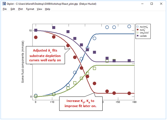
Now adjust KD and KA to improve the fit later on in the experiment. Remember, the half saturation constants describe the inhibition of the reaction rate due to kinetic effects as the substrates are depleted. In this example, your results will not be especially sensitive to the values chosen for KD and KA.
Once you find kinetic parameters that fit the experimental results reasonably well, plot also the
- Biomass concentration, in mg kg−1
- The rate of arsenate reduction, in nmol kg−1 s−1
- The kinetic factors FD and FA, as well as the thermodynamic potential factor FT for the two groups
What are the main controls on the rate of microbial arsenate reduction in our example?
The assemblage of plots below shows our numerical results, plotted together with our experimental data. The first shows concentrations of components in the electron donating reaction, the second those in the electron accepting reaction, and the third shows the effect of growth on the biomass concentration
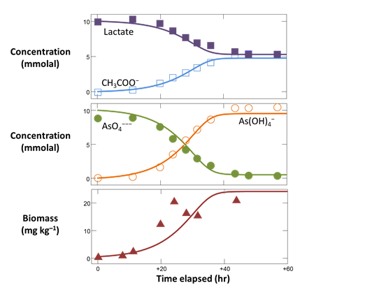
Clearly, the reaction rate increases during the first 30 or so hours, then decreases and eventually stops, even while substrate remains. Plotting the parameters evaluated in our rate law can help us determine the factors controlling reaction rate. The kinetic factors do not deviate from unity until after the thermodynamic potential factor has started to decrease sharply
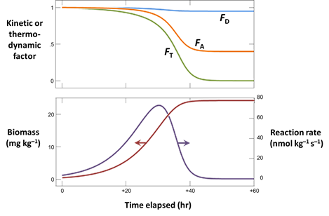
The principal controls on the reaction rate in our example, then, are biomass and thermodynamic drive. Initially, in the presence of abundant lactate and arsenate, the rate is controlled by the size of the microbial population available to catalyze lactate oxidation. As the population increases, so does reaction rate. Later, as reactants are consumed and products accumulate, the reaction approaches the point at which the energy liberated by its progress is balanced by the energy available to drive forward the cellular metabolism, this energy represented by the thermodynamic potential factor FT; over the course of the experiment, the kinetic factors FD and FA play minor roles.
Such a pattern is not typical of microbial metabolisms that exploit more energetically favorable reactions. As the reaction progresses, the rate would likely be controlled by kinetics, rather than thermodynamics.
Task 2: Microbes in an aquifer
Consider two functional groups of microorganisms in an aquifer—sulfate reducers and methanogens—competing for the acetate being produced by fermentation. If seed microbes from the two groups are allowed to grow in the aquifer over time, how do the microbial populations arrange themselves?
The two functional groups of microbes in the aquifer, the sulfate reducing bacteria and methanogens, are present initially in small amounts, but their populations can grow as they derive energy by metabolizing the acetate.
In the example, aquifer sediments are confined by and interleaved with fine-grained sediments that contain sedimentary organic matter. The organic matter decays gradually by microbial fermentation and anaerobic oxidation to simpler compound such as acetate (Ac)
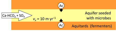
At t = 0, acetate begins to diffuse form the fine-grained layers into the aquifer, where it can serve as the substrate for acetotrophic sulfate reduction

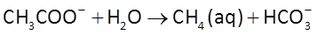
and acetoclastic methanogenesis
The sulfate reducers proceed at a rate r given by the thermodynamically consistent dual Monod equation
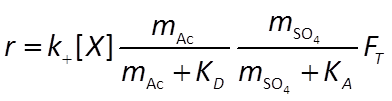
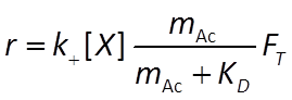
For the methanogens, we use the thermodynamically consistent Monod equation
To model such a scenario, double-click on “Microbes.x1t”. The aquifer considered is 200 km long and water flows through it at a discharge of 10 m3 m−2 yr−1, as you can see on the Domain and Flow panes, respectively. On the Config → Redox Couples… dialog
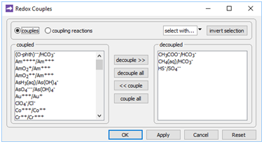
the coupling reactions between carbonate and acetate, carbonate and methane, and sulfate and sulfide are disabled. Configuring the model in this way provides for the redox disequilibrium that supplies sulfate reducers and methanogens with energy.
Select File → View, choose “.\thermo_microbes.tdat” and find “FeO(ox)”. This mineral, which represents the ferrous oxide component in clay minerals, as well as FeS(s) in the subsequent data block have been added to the default thermo dataset. The minerals serve to take up H2S(aq) produced by sulfate reducers

in order to maintain realistic sulfide concentrations in the aquifer.
On Config → Suppress…
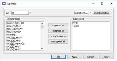
two minerals composed of iron sulfide are excluded from the model, to prevent them from precipitating in place of the FeS(s).
On the Initial pane
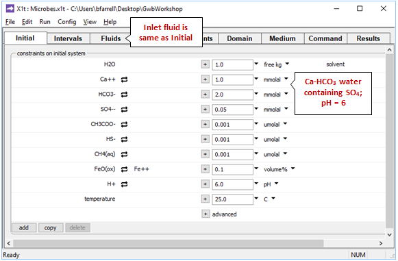
we see the aquifer contains a Ca-HCO3 water of pH 6. The “inlet” fluid (Fluids pane) is of the same composition as the initial groundwater.
The initial and inlet waters contain sulfate, to allow sulfate reducers to respire, as well as arbitrarily small initial amounts of acetate, methane, and sulfide. As discussed, the aquifer sediments contain FeO(ox), a proxy for ferrous iron in clay minerals.
On the Intervals pane
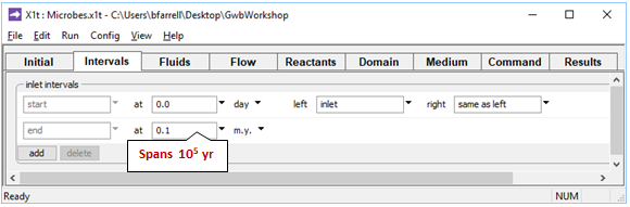
we see the simulation is set to span 105 years, which is sufficient for the microbial populations to adjust to a steady state.
The Reactants pane prescribes the rate at which acetate enters the aquifer
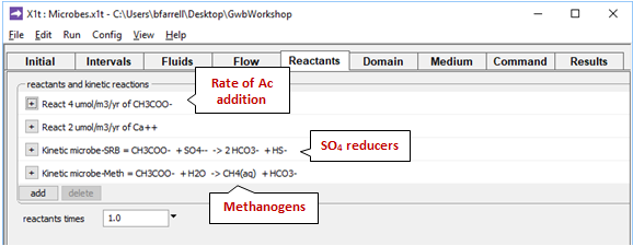
as occurs in nature where the organic matter trapped in fine-grained layers degrades by fermentation.
The pane also contains a data block for the sulfate reducing bacteria, and another for the methanogens. Expanding the block for the sulfate reducers
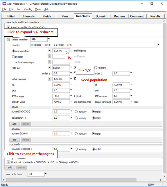
reveals the coefficients in the kinetic rate law, the growth yield and decay coefficient, and the initial microbial population. We specify the average stoichiometric number by setting variable ω (“order1”) to 1/ χ. Expanding the underlying block shows these data for the methanogens.
Take note of the suffix

and execute the model by selecting Run → Go.
When the simulation finishes, plot against position in the aquifer the values at the end of the simulation of the following variables:
- The concentrations of the CH3COO−, SO4−−, and CH4(aq) components in the groundwater, in µmol kg−1
- Biomass concentrations for the sulfate reducers and methanogens, in mg kg−1
- Rates of sulfate reduction and acetoclastis, in mol kg−1 yr−1
- The thermodynamic potential factor FT for the two groups
What factors control the distribution in the aquifer of bacterial sulfate reduction and acetoclastic methanogenesis?
The figures below show the results at the end of the simulation, after groundwater composition and microbial activity across the aquifer have approached a steady state. With time in the simulation, sulfate reducing bacteria grow into a community that consumes sulfate from the recharging groundwater and some of the acetate diffusing into the aquifer
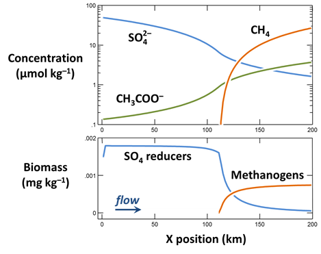
As groundwater flows along the aquifer, its sulfate content is gradually depleted by the sulfate reducers. The acetate added to the aquifer is not entirely consumed by the microbes, so acetate concentration gradually rises. About 100 km along the flowpath, acetate concentration rises to the point at which methanogens can maintain a population.
From this point, sulfate reducers are at a disadvantage. They must compete with methanogens for acetate, and do so in the presence of little sulfate, the paucity of which slows their metabolism. Acetoclastis becomes the dominant metabolism downstream in the aquifer. Methanogens here grow to form a second microbiological zone, which they dominate. The zone is marked geochemically by a rise in acetate concentration and the accumulation in the flowing groundwater of dissolved methane
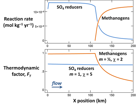
Sulfate reducing bacteria exclude methanogens completely from the upstream portion of the aquifer in an interesting way: they hold acetate concentration to a level at which acetoclastis proceeds at a rate insufficient to allow methanogens to grow as fast as they die.
In order for a population to avoid what ecologists call an “extinction vortex” the growth rate
should not be negative. Where the acetate concentration, mAc, is small, we can simplify the rate law for methanogenesis to
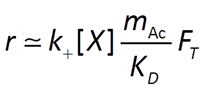
The criterion for maintaining a population of methanogens,
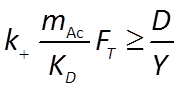
states that mAc must be large enough such that the reaction rate per unit biomass (left side of the inequality) must match the ratio of the decay constant to growth yield. Even in the presence of a strong thermodynamic drive for acetoclastis, the methanogens (because of their low growth yield) cannot colonize this portion of the aquifer.
Authors
Craig M. Bethke and Brian Farrell. © Copyright 2016–2026 Aqueous Solutions LLC. This lesson may be reproduced and modified freely to support any licensed use of The Geochemist's Workbench® software, provided that any derived materials acknowledge original authorship.
References
Bethke, C.M., 2022, Geochemical and Biogeochemical Reaction Modeling, 3rd ed. Cambridge University Press, New York, 520 pp.
Bethke, C.M., B. Farrell, and M. Sharifi, 2026, The Geochemist's Workbench®, Release 18: GWB Reactive Transport Modeling Guide. Aqueous Solutions LLC, Champaign, IL, 191 pp.
Bethke, C.M., D. Ding, Q. Jin and R.A. Sanford, 2008, Origin of microbiological zoning in groundwater flows. Geology 36, 739–742.
Blum, J.S., A.B. Bindi, J. Buzelli, J.F. Stolz and R.S. Oremland, 1998, Bacillus arsenicoselenatis, sp. nov., and Bacillus selenitireducens, sp. nov.: two haloalkaliphiles from Mono Lake, California that respire oxyanions. Archives Microbiology 171, 19–30.
Ingvorsen, K., A.J.B. Zehnder and B.B. Jorgensen, 1984, Kinetics of sulfate and acetate uptake by Desulfobacter postgatei. Applied and Environmental Microbiology 47, 403–408.
Jin, Q. and C.M. Bethke, 2002, Kinetics of electron transfer through the respiratory chain. Biophysical Journal 83, 1797–1808.
Jin, Q. and C.M. Bethke, 2003, A new rate law describing microbial respiration. Applied and Environmental Microbiology 69, 2340–2348.
Jin, Q. and C.M. Bethke, 2005, Predicting the rate of microbial respiration in geochemical environments. Geochimica et Cosmochimica Acta 69 , 1133–1143.
Jin, Q. and C.M. Bethke, 2007, The thermodynamics and kinetics of microbial metabolism. American Journal of Science 307, 643–677.
Jin, Q. and C.M. Bethke, 2009, Cellular energy conservation and the rate of microbial sulfate reduction. Geology 37, 1027–1030.
Oude Elferink, S.J.W.H., A. Visser, L.W. Hulshoff Pol, and A.J.M. Stams, 1994, Sulfate reduction in methanogenic bioreactors. FEMS Microbiology Reviews 15, 119–136.
Pallud, C., and P. Van Cappellen, 2006, Kinetics of microbial sulfate reduction in estuarine sediments. Geochimica et Cosmochimica Acta 70, 1148–1162.
Comfortable with microbial models?
Move on to the next topic, Animation and Video Clips, or return to the GWB Online Academy home.