
Biodegradation
Biodegradation is part of a free web series, GWB Online Academy, by Aqueous Solutions LLC.
What you need:
- GWB Professional recommended
-
Input files:
 Benzene.x1t,
 thermo+benzene.tdat,
 Benzene_Kd.sdat
Download this unit to use in your courses:
- Lesson plan (.pdf)
- PowerPoint slides (.pptx)
Click on a file or right-click and select “Save link as…” to download.
Introduction
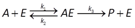
In enzymatic catalysis, a substrate combines with an enzyme to form an activated complex, which can decay to give a catalytic product
The Michaelis-Menten equation gives the rate of forward reaction
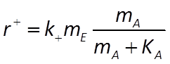
where k+ is the rate constant, mE is enzyme concentration, mA is substrate concentration, and KA = (k2 + k3)/k1 is the half-saturation constant (molal).
The effect of substrate concentration mA on the rate predicted by this equation follows a characteristic pattern, as can be seen from the figure below.
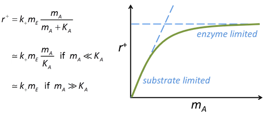
Where substrate concentration is considerably smaller than the half-saturation constant, the reaction rate is proportional to mA. In other words, it is substrate limited. For the opposite case, reaction rate is invariant with respect to substrate concentration.
The Michaelis-Menten equation behaves very much like the Langmuir and Monod equations, described in the Surface Complexation and Microbial Populations sections, respectively.
In geochemical modeling, we prefer rate laws giving the net rather than the forward reaction rate. Accounting for the reverse reaction,
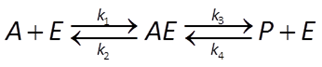
the net rate proceeds at the rate of the forward less the reverse reaction. It is given by
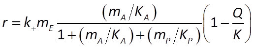
where mP is product concentration, KP = (k2 + k3)/k4 is the half-saturation constant for the reverse reaction, and Q and K are the reaction's activity product and equilibrium constant, respectively.
Task 1: Biodegradation of benzene
We consider here the fate and transport in aerobic groundwater of the ring compound benzene, C6H6. Benzene is a suspected carcinogen with an MCL (Maximum Contamination Level) set by the US Environmental Protection Agency of 5 µg kg−1.
Benzene is perhaps the most commonly remediated groundwater contaminant because it makes up much of the volatile fraction of petroleum fuels. Contamination of this sort is commonly called BTX, after the most soluble compounds—benzene, toluene, xylene—that make up gasoline. There are approximately 100,000 sites in the US known to be contaminated with BTX.
Dissolved in groundwater, benzene is gradually degraded by a variety of microorganisms present naturally in the subsurface. The natural attenuation is most rapid under aerobic conditions.
To compute a model of aerobic biodegradation in flowing groundwater, double-click on file “Benzene.x1t”. Program X1t, the one-dimensional reactive transport model in the GWB, opens.
Click on File → View → “.\thermo+benzene.tdat”. This dataset is the “thermo.tdat” compilation installed with the software, with an added entry for benzene (learn how to edit the thermo dataset yourself). Look for "Benzene(aq)" to find the reaction
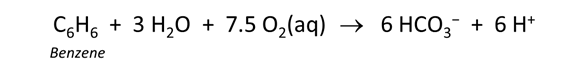
Considering the log K at 25°C of 537.5, should we expect benzene oxidation to be a favored reaction under aerobic conditions?
Open the Config → Redox Couples… dialog
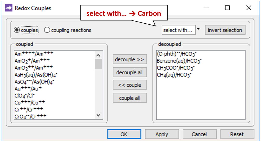
and note that the reactions between carbonate and the organic forms of carbon have been disabled. Carbon in the simulation can therefore change redox state only by kinetic reaction.
Look at the Initial pane
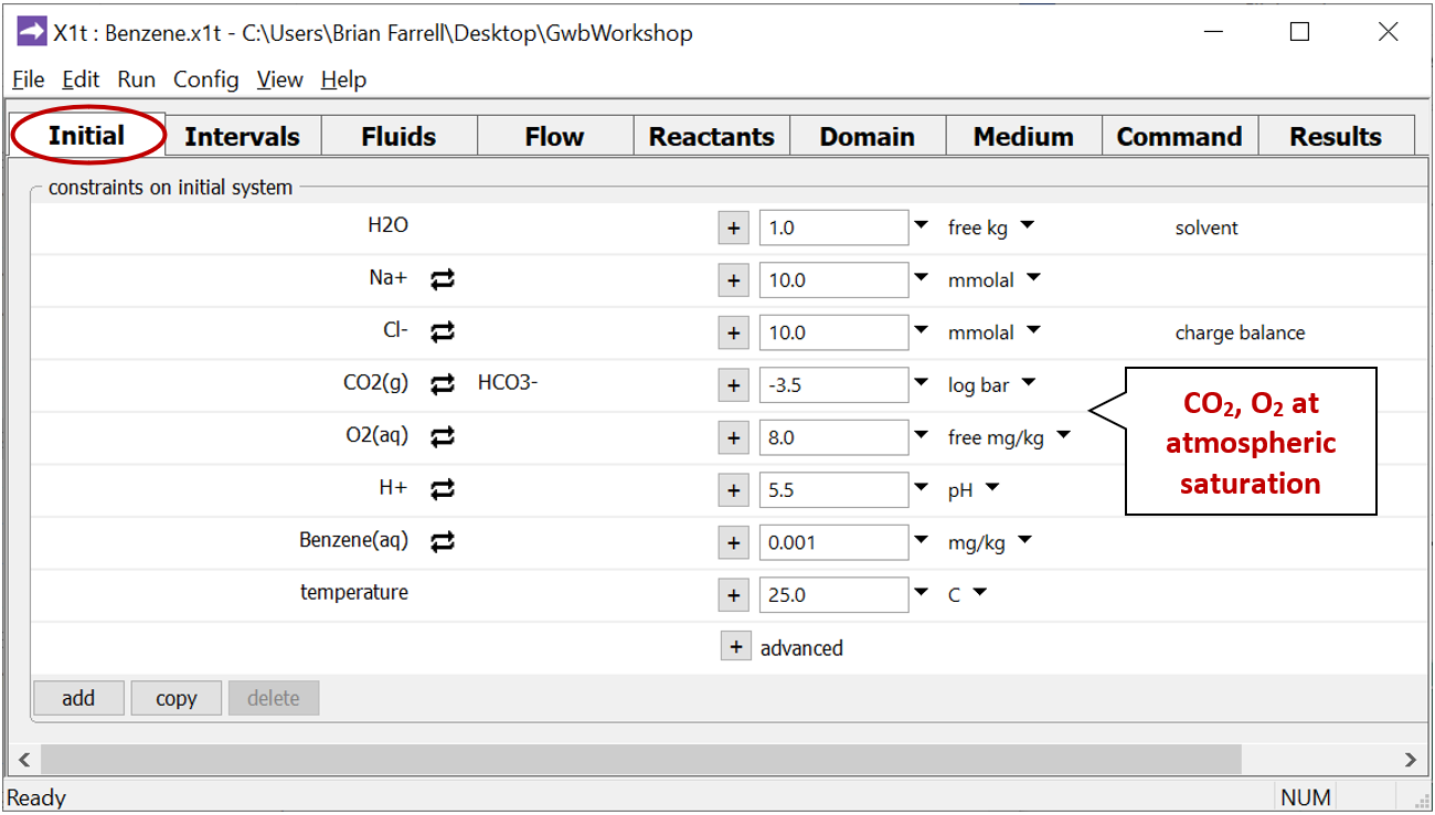
to see the composition of water in the aquifer at the start of the simulation.
The Fluids pane shows the two waters that will pass into the domain. The “contaminated” fluid
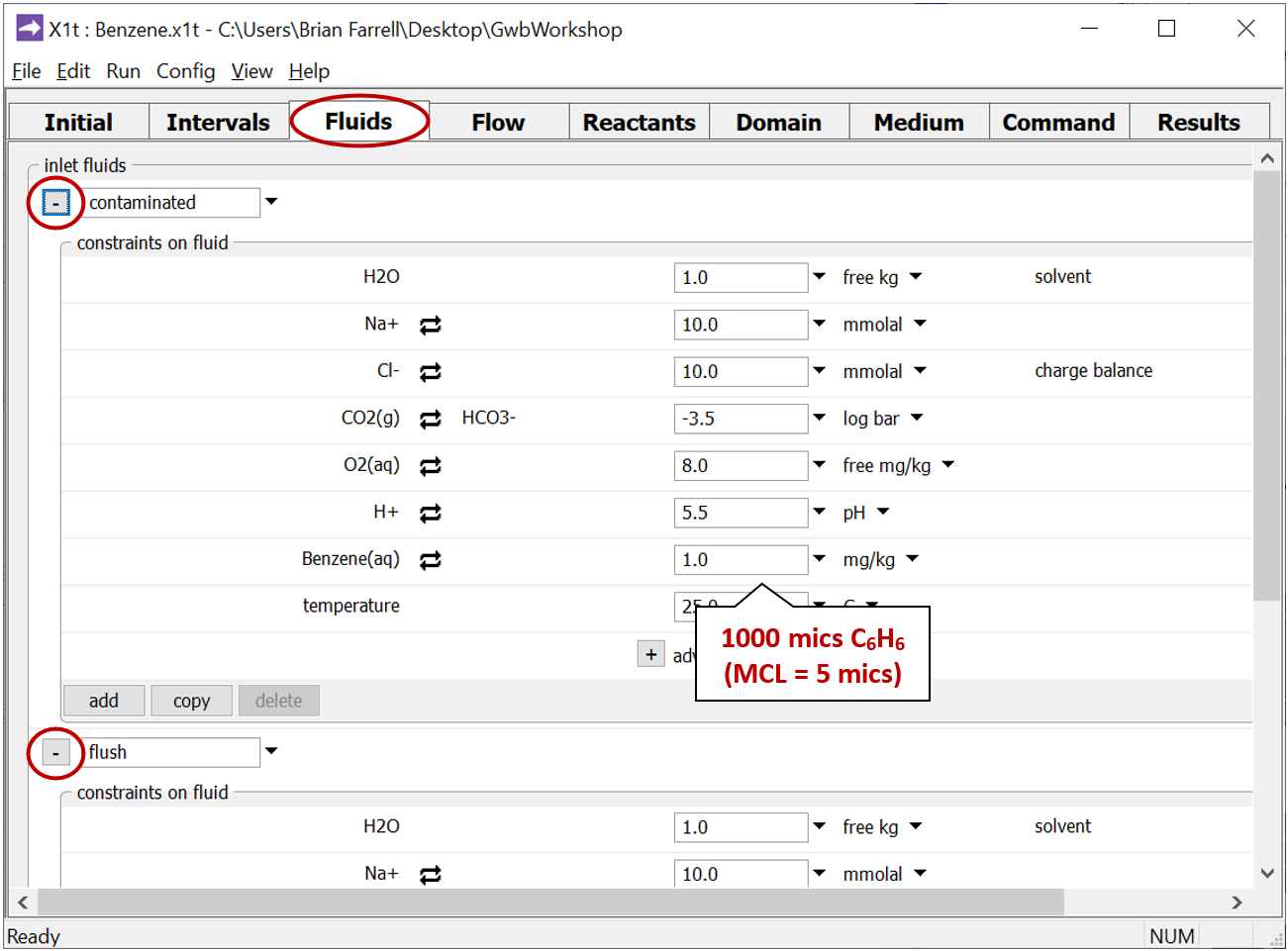
contains 1000 µg kg−1 benzene, while the “flush” fluid holds the clean water that later flushes the aquifer, after it's been contaminated.
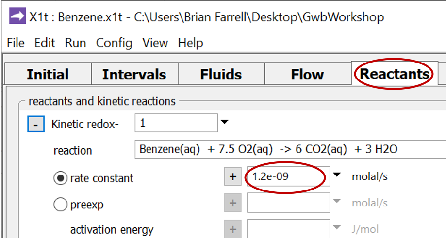
Move to the Reactants pane and expand the entry for reactant “redox-1”
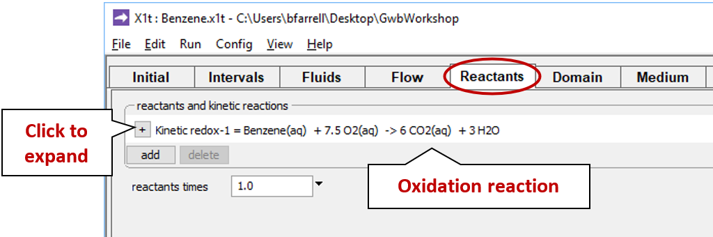
This entry sets the aerobic mineralization of benzene as a kinetic reaction
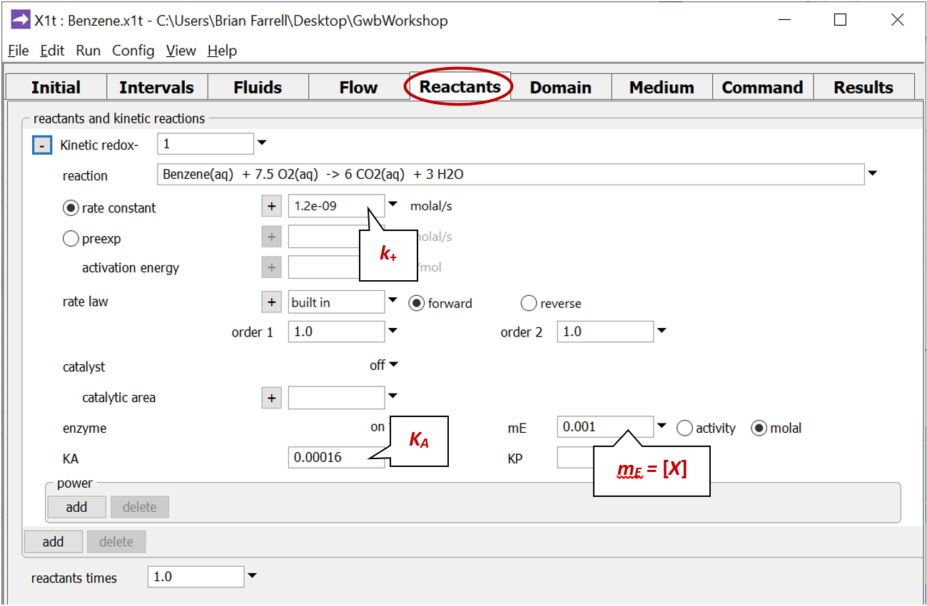
and specifies values for the parameters in the corresponding rate law. If the kinetic reaction hadn't already been created, you would click on  → Kinetic → Redox reaction to do so.
Note on Config → Output… a suffix “_benzene” has been applied

Select Run → Go to trace the simulation.
To compute the non-reacting case, return to the Reactants pane
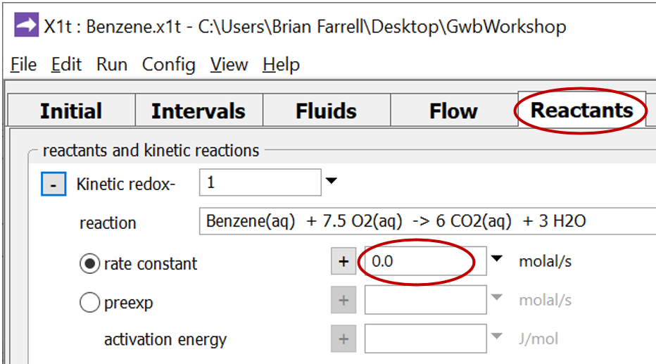
and set the kinetic rate constant k+ to 0. The null entry disables the reaction. Set a different suffix

and rerun the model.
Graph your results by double-clicking on the output files “X1t_plot_benzene.xtp” and “X1t_plot_benzene0.xtp”. How, according to the model, does biodegradation affect benzene migration?
The plot below shows the results of the non-reacting and biodegrading cases together. The non-reacting case, in blue, is much like the example from the Mass Transport section. The pulse of benzene migrates at the rate of groundwater flow, traversing the aquifer in 10 years
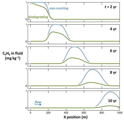
Where benzene can degrade, the concentration attenuates as the pulse travels through the domain. The pulse is asymmetrical because the benzene at the leading edge has been in the domain longer, and hence has been degrading for a longer period of time.
Task 2: Sorption and biodegradation
In aquifers containing significant amounts of natural organic matter, benzene sorbs to the surfaces of the organic particles, retarding its migration. The amount of retardation varies with organic content.
To model in X1t how sorption might affect benzene biodegradation, restore the rate constant for benzene bio-oxidation
if necessary, and read in (or drag into the window) the surface dataset “Benzene_Kd.sdat”
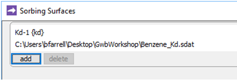
The dataset specifies a distribution coefficient Kd' of .16 × 10−3 (mol C6H6) (g sediment)−1. This value corresponds to a retardation factor RF of 2, which might be observed in an aquifer containing about 1 wt% organic matter.
Close the dialog, set a new suffix

and rerun the simulation.
How does sorption affect the mobility of benzene contamination, compared to the non-sorbing case? In which case does benzene biodegrade most rapidly? Why?
The plot below shows the sorbing and biodegrading case, in orange, together with our previous results
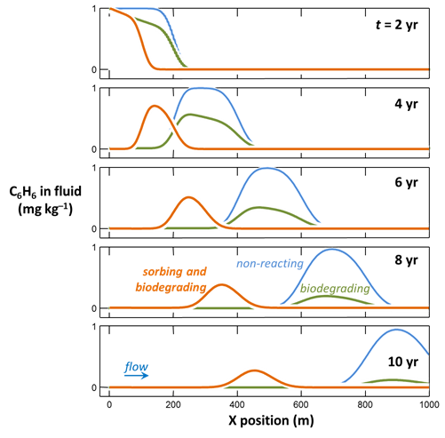
The benzene passes more slowly through the aquifer, moving at only half the speed of the groundwater flow, reflecting sorption and retardation. Less benzene degrades by biological activity than in the non-sorbing case, since at any given time only a fraction of the contaminant is available to the microbial consortium in aqueous form.
Animation of two-dimensional example
This clip follows a plume of benzene contamination as it moves through a heterogeneous aquifer and is degraded by the microbial community there. The simulations show:
- The non-degrading case, for reference
- The case of biodegradation in the absence of sorption
- A simulation in which the benzene both sorbs and biodegrades
Authors
Craig M. Bethke and Brian Farrell. © Copyright 2016–2026 Aqueous Solutions LLC. This lesson may be reproduced and modified freely to support any licensed use of The Geochemist's Workbench® software, provided that any derived materials acknowledge original authorship.
References
Alvarez, P.J.J., P.J. Anid and T.M. Vogel, 1991, Kinetics of aerobic biodegradation of benzene and toluene in sandy aquifer material. Biodegradation 2, 43–51.
Bethke, C.M., 2022, Geochemical and Biogeochemical Reaction Modeling, 3rd ed. Cambridge University Press, New York, 520 pp.
Bethke, C.M., B. Farrell, and M. Sharifi, 2026, The Geochemist's Workbench®, Release 18: GWB Reactive Transport Modeling Guide. Aqueous Solutions LLC, Champaign, IL, 191 pp.
Comfortable with biodegradation models?
Move on to the next topic, Dissolution and Precipitation, or return to the GWB Online Academy home.