Dissolution and precipitation

Jump to:

Introduction Task 1: Quartz weathering Animation of two-dimensional example Authors and references

Dissolution and Precipitation is part of a free web series, GWB Online Academy, by Aqueous Solutions LLC.

What you need:

GWB 2023 Professional recommended
Input file: Quartz.x1t

Download this unit to use in your courses:

Lesson plan (.pdf)
PowerPoint slides (.pptx)

Click on a file or right-click and select “Save link as…” to download.

Introduction

The GWB programs have a Built-in Rate Law for mineral dissolution and precipitation

Built-in rate law

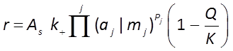
where r is the mineral's dissolution rate, A_S is the surface area of the mineral, k₊ is the intrinsic rate constant, a_j, m_j are the activity or concentration of promoting or inhibiting species, P_j is a species' power (+ is promoting, − is inhibiting), and Q and K are the activity product and equilibrium constant, respectively, for the dissolution reaction.

The user supplies parameters for the rate law, including a specific surface area and rate constant for each mineral. The rate constant can be set directly or it can be calculated from the activation energy E_A and pre-exponential factor A using the Arrhenius equation

Arrhenius equation

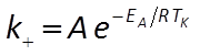
where R is the gas constant, and T_K is absolute temperature.

Task 1: Quartz weathering

How rapidly does mineral dissolution affect the chemistry of water flowing along an aquifer composed of only quartz? Double-click on “Quartz.x1t” to calculate a reactive transport model of rainwater infiltrating such an aquifer.

The Initial pane

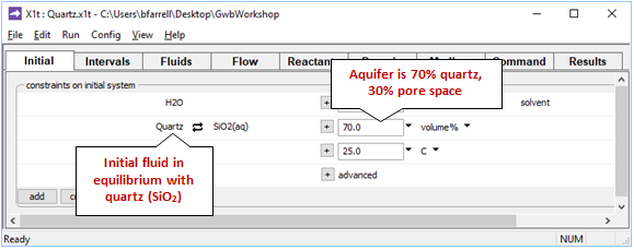
shows the conditions at the onset of the simulation.

On the Intervals pane

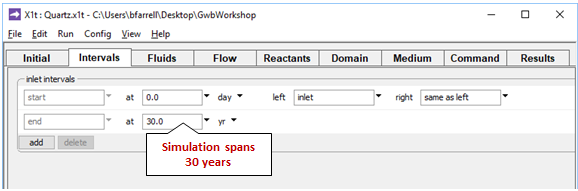
we set the model's time span and associate an inlet fluid with the domain's left side.

On the Fluids pane

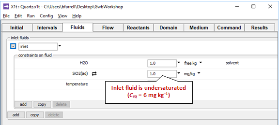
we define a fluid called “inlet”, the rainwater recharging the aquifer, which is set to be undersaturated with respect to quartz.

On the Reactants pane a kinetic law governs quartz dissolution

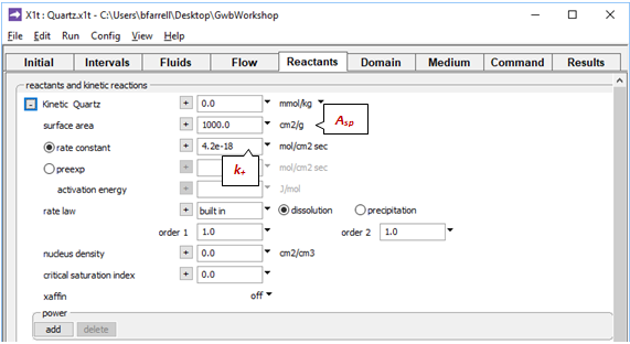
The rate constant k₊ is from Rimstidt and Barnes (1980), and the specific surface area A_sp is from Leamnson et al. (1969). The mass of quartz carried in the simulation is the amount of buffering mineral shown in the Initial pane, plus the mass set in the Reactants pane, which here is 0.

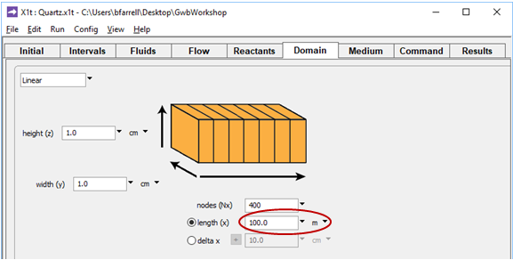
On the Domain pane, aquifer length is set to “100 m”

and on the Flow pane

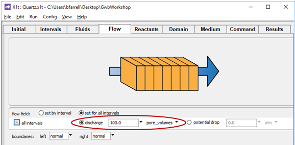
the simulation is configured to displace the pore fluid in the aquifer 100 times. Because the simulation spans 30 years, groundwater velocity v_x is (100 m)/(30 yr/100), or 330 m yr⁻¹.

Note the suffix

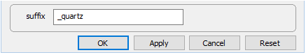
and select Run → Go to calculate the model.

On the Results pane, click on and graph the concentration in mg kg⁻¹ of SiO₂(aq) in the fluid against position in the aquifer. Choose the time step at the end of the simulation, t = 30 years.

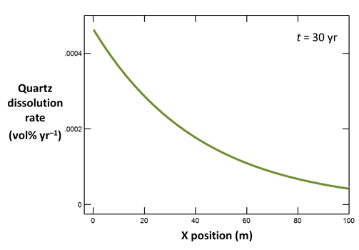
Return to X1t and click on once again to open a second instance of Xtplot. Plot along the aquifer the dissolution rate (on Y Axis pane, set “Variable type” to “Reactant properties”, then choose “Dissolution rate, Quartz”) in volume percent of the aquifer per year, again at t = 30 yr.

How does quartz dissolution affect silica concentration in the flowing groundwater? How does silica accumulating in the groundwater affect the distribution of the quartz dissolution reaction?

The plot below shows the concentration of silica dissolved in a portion of the aquifer extending 100 m from the recharge point

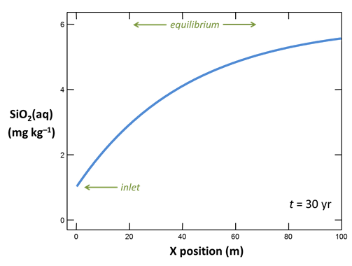
In the first few meters, the fluid has not yet dissolved much quartz, so the concentration is similar to that of the recharging fluid. The concentration increases with distance, approaching the equilibrium value (quartz solubility) 100 m from the recharge point.

Plotting dissolution rate against position, it is evident that reaction is most rapid near the recharge point and decreases along the direction of flow as dissolved silica accumulates in the groundwater

In the figure below, the dissolution rate is plotted against time at a location 5 m from the recharge point. As rainwater enters the aquifer and reaction begins at that point, the dissolution rate, initially 0, quickly adjusts to an almost constant value, as does silica concentration

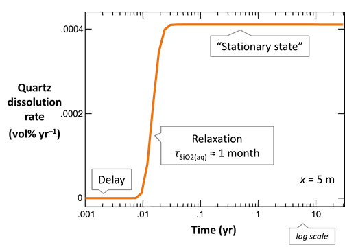
The simulation end result is not a steady state, strictly speaking, because quartz is gradually dissolving, decreasing its surface area and causing the dissolution rate to diminish slowly with time.

Leaving the two instances of Xtplot alive, return to X1t and increase the time span

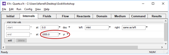
from 30 to 1000 years. This change has the effect of prescribing slower groundwater flow, since the pore fluid will still be displaced 100 times. Now, v_x = (100 m)/(1000 yr/100) = 10 m yr⁻¹.

Rerun the simulation. When the calculation finishes, the graphs you made in Xtplot will update themselves automatically. How has the distribution of the silica dissolution reaction changed in the aquifer?

Finally, repeat the calculation assuming a time span of 1 year, which corresponds to v_x = 10, 000 m yr⁻¹. How have your plots changed?

The figure below shows results calculated for velocities spanning the range considered. The simulations correspond to Damköhler numbers Da much less than 1 for rapid flow, to much greater than 1 when flow is slow

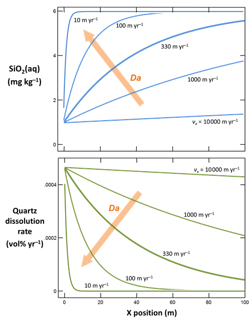
At low Da, transport overwhelms reaction and the fluid across the domain remains fully undersaturated with respect to quartz. Since quartz saturation changes little with position, the dissolution rate remains nearly constant. At high Da, in contrast, reaction controls transport and the infiltrating rainwater reacts toward equilibrium before migrating far from the inlet. In this case, the reaction rate is nearly 0 across most of the domain.

Only for the intermediate cases does silica concentration and reaction rate vary greatly across the main part of the domain. Significantly, only these cases benefit from the extra effort of calculating a reactive transport model.

For more rapid flows, the same result is given by a lumped parameter simulation, or box model, as we could construct in React. And for slower flow, a local equilibrium model suffices.

Animation of two-dimensional example

In an application of mineral dissolution and precipitation kinetics, hot water is injected into a petroleum reservoir in order to stimulate production. The steam flood reacts with kaolinite, calcite, and quartz in the formation to produce swelling clay (beidellite) and CO₂.

The animations in the clip show variation over the course of the flood in:

Temperature
CO₂ fugacity
Percent swelling clay
Formation permeability, accounting for the clay produced

Authors

Craig M. Bethke and Brian Farrell. © Copyright 2016–2024 Aqueous Solutions LLC. This lesson may be reproduced and modified freely to support any licensed use of The Geochemist's Workbench® software, provided that any derived materials acknowledge original authorship.

References

Bethke, C.M., 2022, Geochemical and Biogeochemical Reaction Modeling, 3^rd ed. Cambridge University Press, New York, 520 pp.

Bethke, C.M., B. Farrell, and M. Sharifi, 2024, The Geochemist's Workbench®, Release 17: GWB Reactive Transport Modeling Guide. Aqueous Solutions LLC, Champaign, IL, 191 pp.

Knapp, R.B., 1989, Spatial and temporal scales of local equilibrium in dynamic fluid-rock systems. Geochimica et Cosmochimica Acta 53, 1955–1964.

Lasaga, A.C. and D.M. Rye, 1993, Fluid flow and chemical reaction kinetics in metamorphic systems. American Journal of Science 293, 361–404.

Leamnson, R.N., J. Thomas, Jr. and H.P. Ehrlinger, III, 1969, A study of the surface areas of particulate microcrystalline silica and silica sand. Illinois State Geological Survey Circular 444, 12.

Rimstidt, J.D. and H.L. Barnes, 1980, The kinetics of silica-water reactions. Geochimica et Cosmochimica Acta, 44 1683–1700.

Comfortable with mineral dissolution and precipitation?

Move on to the next topic, Microbial Populations, or return to the GWB Online Academy home.