
Geothermometry
Geothermometry is part of a free web series, GWB Online Academy, by Aqueous Solutions LLC.
What you need:
- GWB Standard recommended
-
Input files:
 geotherm.rea,
geotherm2.rea, Hveravik.rea
geotherm.rea,
geotherm2.rea, Hveravik.rea
Download this unit to use in your courses:
- Lesson plan (.pdf)
- PowerPoint slides (.pptx)
Click on a file or right-click and select “Save link as…” to download.
Introduction
In this lesson we use geochemical modeling to estimate the temperatures at which natural fluids have equilibrated in the subsurface. This field of study is known as geothermometry.
In the first part of the lesson we simulate how a hypothetical groundwater behaves chemically as it is sampled at depth and cooled. We use React to test the temperatures at which various minerals are in equilibrium with the fluid to see how well we can estimate the sampling temperature. Later, we apply geothermometric techniques to interpret chemical analyses of natural waters.
Task 1: Principles of geothermometry
First, we simulate sampling a hypothetical geothermal water at 250°C and letting it cool to room temperature.
Double-click on file "geotherm.rea", and when React opens, look at the Basis pane
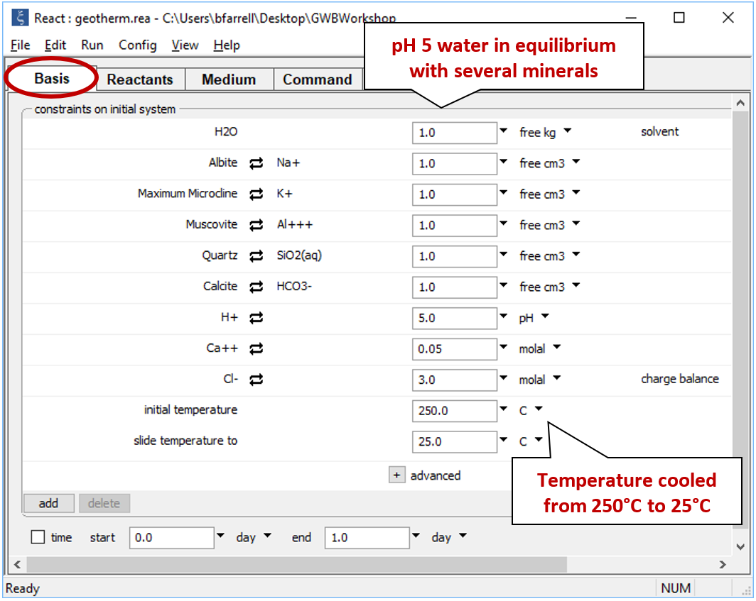
The Basis pane contains a fluid initially in equilibrium with albite, muscovite, quartz, potassium feldspar (maximum microcline), and calcite at 250°C. In addition to the initial temperature, we've set a final temperature (“slide temperature to”), so the program will trace a simple polythermal reaction path over which the fluid cools gradually to room temperature.
On the Config → Stepping… dialog
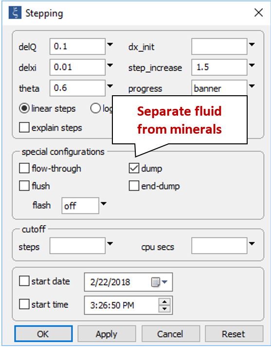
we see the “dump” command has been selected. This setting removes minerals from the initial system, simulating separation of the fluid from reservoir minerals as it is sampled.
On the Config → Options… dialog
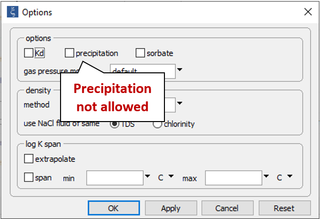
we see the “precipitation” option has been deselected. This setting prevents the program from allowing minerals to precipitate. In practice, samples are quickly acidified after they have been sampled and their pHs determined. Preservation by this procedure keeps solutes from precipitating and altering the fluid's composition before analysis.
On Config → Output… set a suffix "_geotherm"

Click OK, then on the main window select Run → Go.
Plot how pH and CO2(g) partial pressure vary with temperature. Why do these values change as the fluid cools? Would you expect CO2(g) to effervesce from the fluid as it's brought to room conditions?
The fluid's pH changes with temperature from its initial value of 5 at 250°C to less than 4 at 25°C
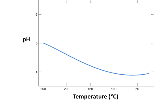
The change is due entirely to variation in the stabilities of the aqueous species in solution. As shown below, the H+ concentration increases in response to the dissociation of the HCl ion pair and the breakdown of CO2(aq)
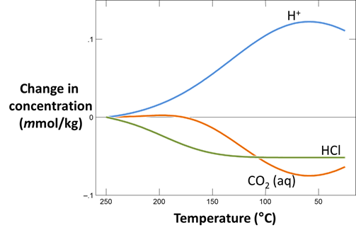
The figure above is what's called a delta plot. For each variable, the difference from its original value is plotted. A positive value indicates that the concentration has increased from its initial value with reaction progress, while a negative value indicates a decrease in concentration.
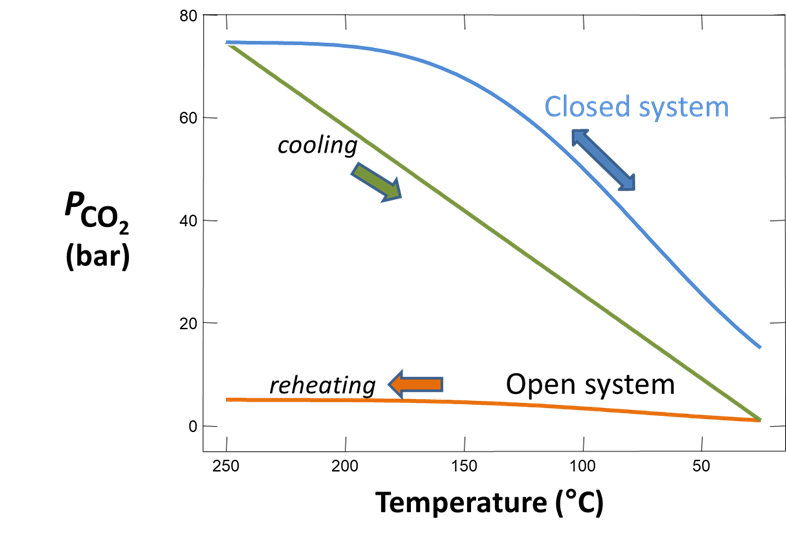
The CO2 partial pressure decreases sharply during cooling, as would be expected, since gas solubility increases as temperature decreases
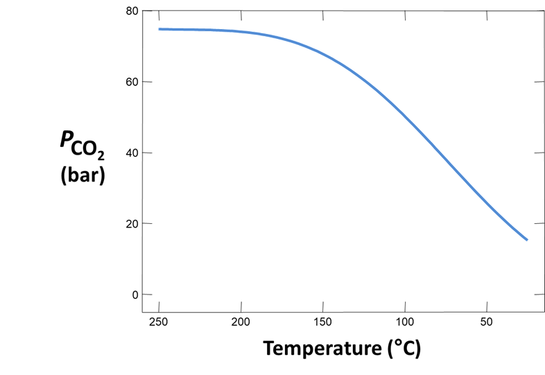
Because of its high partial pressure, CO2(g) would almost certainly effervesce from the fluid.
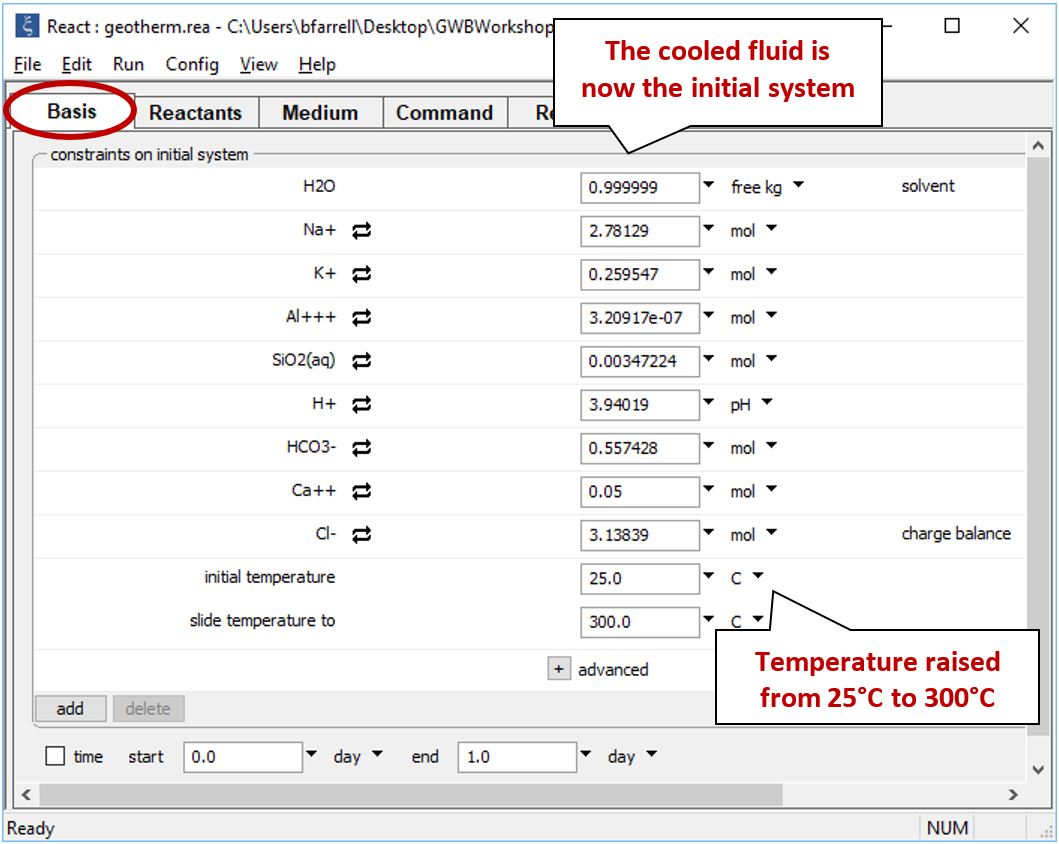
Now, let's take our sampled fluid and use it to predict its original temperature (which we already know, since we synthesized the fluid in the first place).
We'll take our result from the previous run and reverse the reaction path by reheating the fluid to 300°C. Go to Run → Pickup → System → Fluid. Click on the unit pulldown next to the “temperature” field, select the “sliding temperature” option, and set a value of “300°C” in the “slide temperature to” field that appears
Run the simulation, then diagram the saturation states of albite, quartz, muscovite, maximum microcline, and calcite (note that all but the latter contain SiO2) against temperature. At what temperature was the fluid in equilibrium with these minerals? Have we successfully predicted, in this hypothetical case, the fluid's original temperature?
Plot the saturation states of several minerals not included in the initial system. Can you guess whether a mineral is likely to be found in the formation from which the fluid was sampled?
The results for the cooling and reheating paths are plotted together below
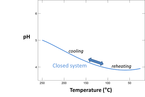
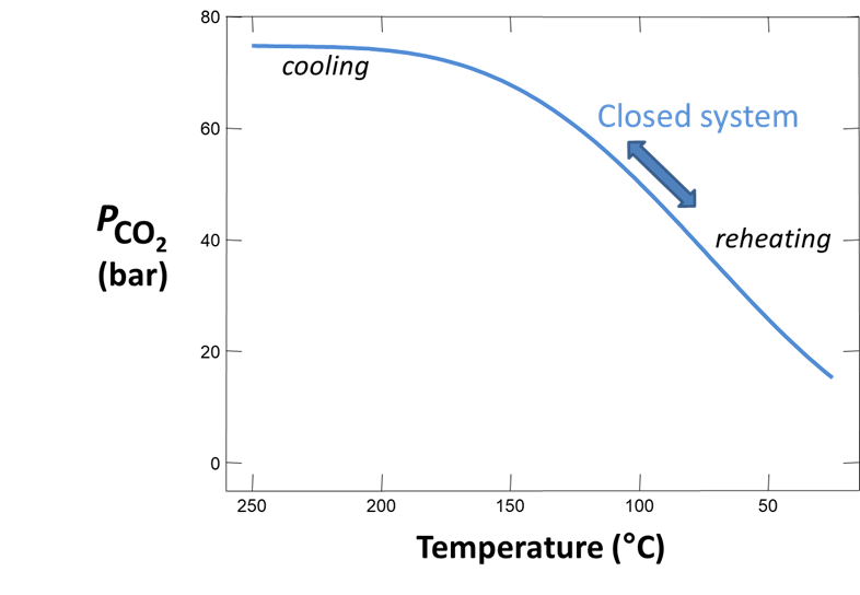
Upon reheating the fluid, the values predicted for pH and CO2 partial pressure retrace the paths followed during the cooling calculation. Since the system is closed to mass transfer, its equilibrium state depends only on temperature.
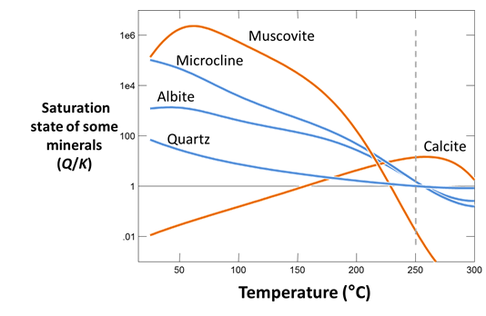
The figure below shows the saturation indices calculated for various minerals
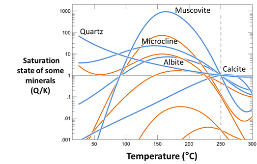
Each of the minerals (albite, muscovite, quartz, potassium feldspar, and calcite, plotted in blue) present in the formation when the fluid was sampled is in equilibrium (i.e., log Q/K = 0) at 250°C. The minerals are in equilibrium at no other temperature. Minerals in the database that were not present in the formation (plotted in orange) appear undersaturated at the equilibrium temperature. These two criteria allow us to uniquely identify the fluid's original temperature.
Task 2: Cooling in an open system
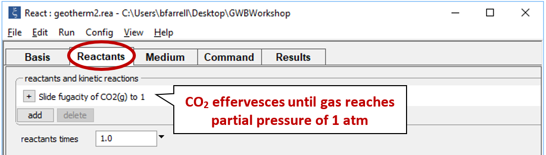
As a second experiment, let's sample the same fluid but allow it to effervesce CO2(g) until the gas reaches a partial pressure of 1 atmosphere. We'll start as before, but this time we'll include a slide command to vary the CO2(g) fugacity.
Double-click on file "geotherm2.rea", and when React opens, move to the Reactants pane
Set a suffix "_geotherm2" and run the simulation.
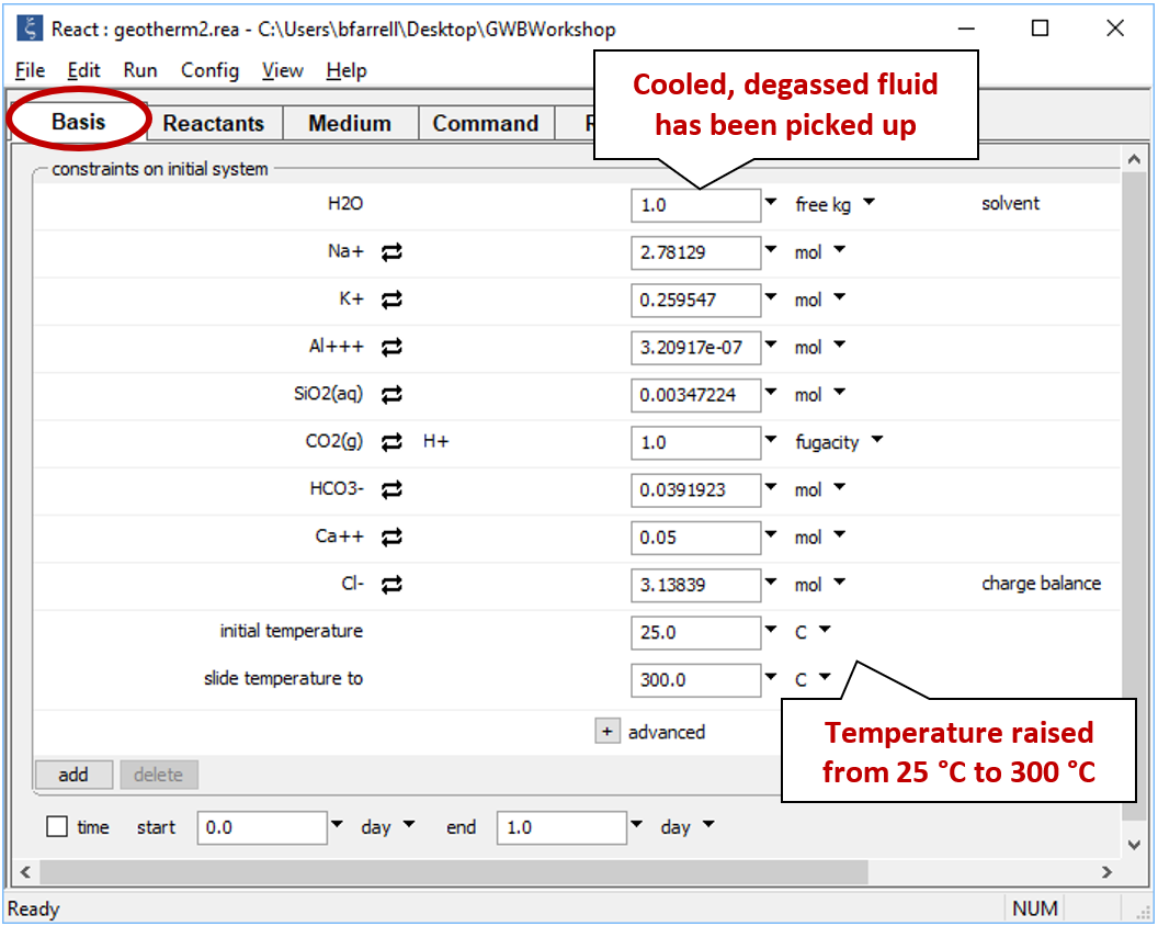
As before, go to Run → Pickup → System → Fluid to pick up the result of the previous calculation, then select the “sliding temperature” option and set the target temperature to “300°C” using the “slide temperature to” field
After you've run the simulation, plot mineral saturation versus temperature, as before. Why do the results of this run differ from those of the previous run? How does the temperature that you might predict by plotting mineral saturation compare to the fluid's actual initial temperature?
In the open system, the CO2 partial pressure varies linearly over the reaction path from 75 bar to a value of about 1, as we prescribed, tracing a path of lower partial pressure than prescribed for the closed system. To maintain the lower partial pressure, the program allows CO2 to escape from the fluid into the external gas buffer
The pH follows a path of higher values than in a closed system, reflecting the loss of CO2, an acid gas
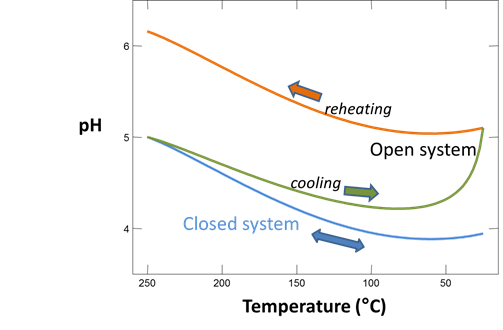
Upon reheating the fluid, neither the pH nor CO2 partial pressure returns to its original value at 250°C.
The predicted saturation states of the formation minerals, furthermore, no longer identify a unique formation temperature. Whereas the temperatures suggested by albite, quartz, and potassium feldspar are quite close to the 250°C formation temperature, those predicted by assuming that the fluid was in equilibrium with muscovite and calcite are too low
To avoid errors of this sort, we would need to determine the amount of gas lost from the sample and reintroduce it to the equilibrium system before calculating saturation indices.
Task 3: Application to natural waters
We'll try to apply geothermometry to natural waters from the geothermal areas of Iceland. Hot groundwaters in these areas, derived from basaltic rocks in or near active volcanic belts, provide a primary energy resource for the island.
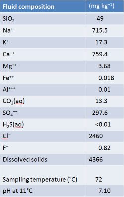
The table below, from Arnorsson et al. (1983), shows the composition and low-temperature pH of the effluent from a hot spring in Hveravik. The water discharges at 72°C
The origin of the spring water is unknown. Does it circulate at high temperature but cool at the discharge point? Is it hot saline water from depth that has mixed with local groundwater near the spring (and hence likely to be out of equilibrium with most minerals)? Has it degassed significantly as it discharged and hence lost its original chemistry? Or is it a relatively shallow groundwater that has reached equilibrium with its host rock at about its discharge temperature?
Open file “Hveravik.rea” and look at the Basis pane
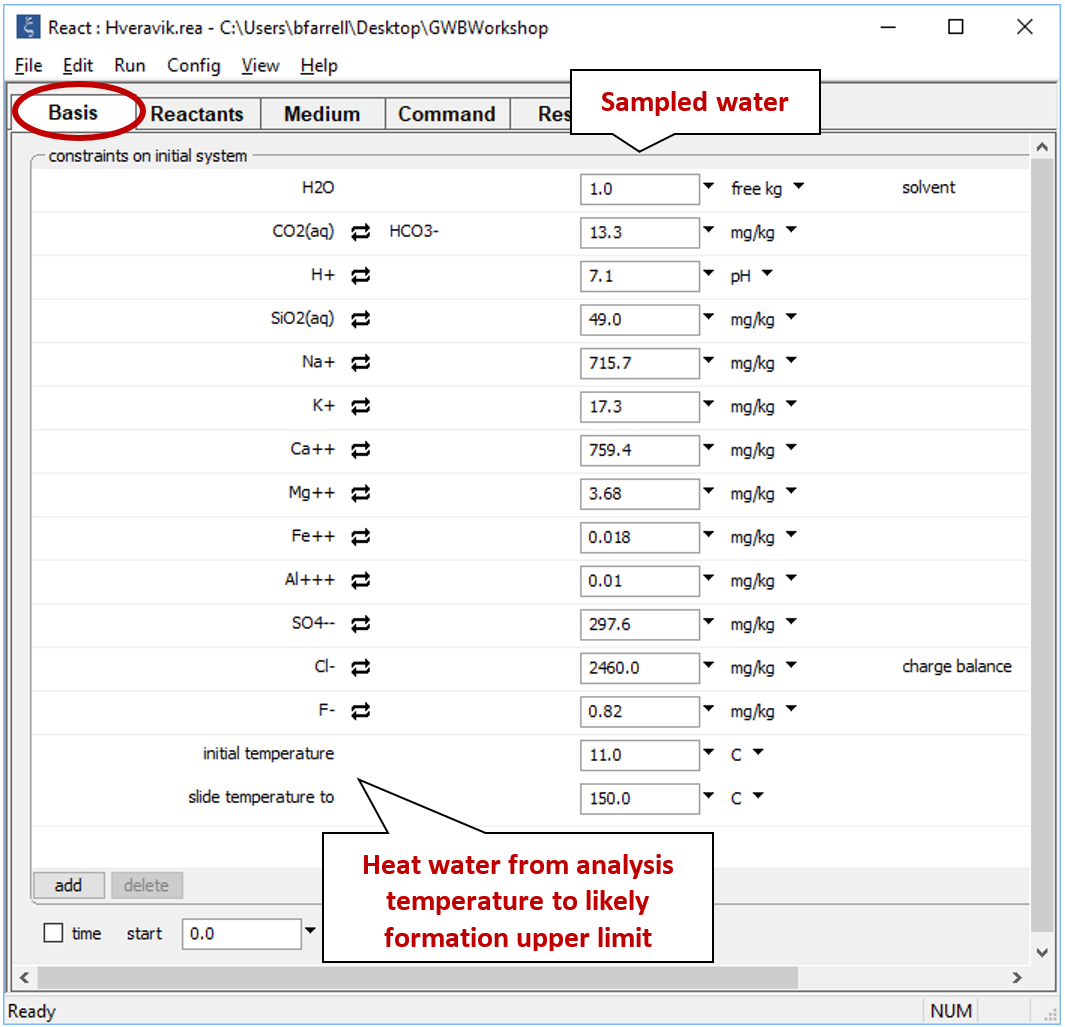
The redox state of the fluid is likely rather oxidizing since there is much more sulfate than sulfide. The exact oxidation state is unknown, however, because H2S was not detected in the analysis. For this reason, we won't consider redox reactions in our calculations. We've set a sliding temperature path which will carry the fluid to 150°C, a likely upper bound on temperature.
On the Config → Options... dialog
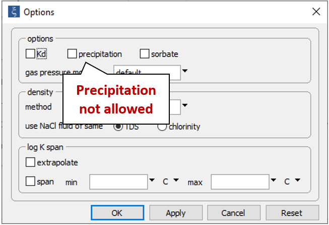
the precipitation option has been deselected.
On Config → Output... set a suffix “_Hveravik”

Click OK, then on the main window select Run → Go.
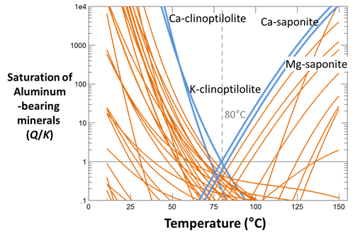
Plot the saturation states in the fluid of all aluminum minerals. At what temperature do you think the fluids equilibrated in the subsurface?
We can limit our plot of mineral saturations to aluminum-bearing minerals by selecting “Al+++” from the pulldown next to “Consider”. Many minerals are supersaturated at low and high temperatures, but a clear equilibrium point appears at about 80°C, slightly warmer than the discharge temperature of 72°C. At this point, the fluid's composition seems to be controlled by calcium and potassium clinoptilolite (zeolites; e.g., CaAl2Si10)24 · 8H2O) and calcium and magnesium saponite [smectite clays; e.g., Ca.165Mg3Al.33Si3.67O10(OH)2] minerals
Plot the saturation states of the silica polymorphs quartz, cristobalite, chalcedony, tridymite, and amorphous silica. With which silica mineral has the fluid equilibrated at the temperature suggested by aluminosilicate equilibria? What temperature would the quartz geothermometer (equilibrium with quartz) predict?
Chalcedony and tridymite are close to equilibrium with the fluid at 80°C, the temperatue suggested by equilibrium with the aluminosilicate minerals. Opal-CT, an interlayering of chalcedony and tridymite with a stability falling between the two minerals, is likely the silica mineral to have equilibrated with the fluid, though it is not accounted for in our simulation
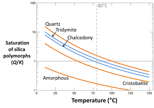
The fluid's equilibrium temperature with quartz is about 100°C. Quartz, however, is commonly supersaturated in geothermal waters below 150°C, so it can give erroneously high equilibrium temperatures when applied in geothermometry.
In light of your results, does degassing seem to have affected the fluid's chemistry? Speculate on the origin of the fluid, considering the information above, the amount of dissolved solids in the fluid, and the fluid's oxidation state.
Authors
Craig M. Bethke and Brian Farrell. © Copyright 2016–2026 Aqueous Solutions LLC. This lesson may be reproduced and modified freely to support any licensed use of The Geochemist's Workbench® software, provided that any derived materials acknowledge original authorship.
References
Arnorsson, S., E. Gunnlaugsson and H. Svavarsson, 1983, The chemistry of geothermal waters in Iceland, II. Mineral equilibria and independent variables controlling water compositions. Geochimica et Cosmochimica Acta 47, 547–566.
Bethke, C.M., 2022, Geochemical and Biogeochemical Reaction Modeling, 3rd ed. Cambridge University Press, New York, 520 pp.
Bethke, C.M., B. Farrell, and M. Sharifi, 2026, The Geochemist's Workbench®, Release 18: GWB Reaction Modeling Guide. Aqueous Solutions LLC, Champaign, IL, 219 pp.
Comfortable with geothermometry?
Move on to the next topic, Fluid Mixing and Scaling, or return to the GWB Online Academy home.