
Fluid mixing and scaling
Fluid Mixing and Scaling is part of a free web series, GWB Online Academy, by Aqueous Solutions LLC.
What you need:
- GWB Standard recommended
-
Input files:
 flashBa++.rea,
flashSO4--.rea,
flashBa++.rea,
flashSO4--.rea,
 sulfate_scaling.gss
Download this unit to use in your courses:
- Lesson plan (.pdf)
- PowerPoint slides (.pptx)
Click on a file or right-click and select “Save link as…” to download.
Introduction
Petroleum engineers use a variety of flooding agents to displace fluids and increase production from oil and gas reservoirs, including seawater, hot water, acids, carbon dioxide, and alkali solutions. In some cases, the injected fluid is used as a drive to sweep oil through the reservoir or up the wellbore. Other fluids are intended to react directly with the reservoir mineral or fluids to increase permeability or improve oil mobility.
The floods, which are generally far from chemical equilibrium with sediments in the reservoir, are likely to react extensively once they enter the formation, causing some minerals to dissolve and others to precipitate as cement. Hutcheon (1984) appropriately refers to this process as artificial diagenesis.
Task 1: Fluid mixing
You can use React to create “flash diagrams” showing the result of mixing two fluids in all possible mixing ratios. Double-click on file “flashBa++.rea”, and when React opens, go to the Basis pane
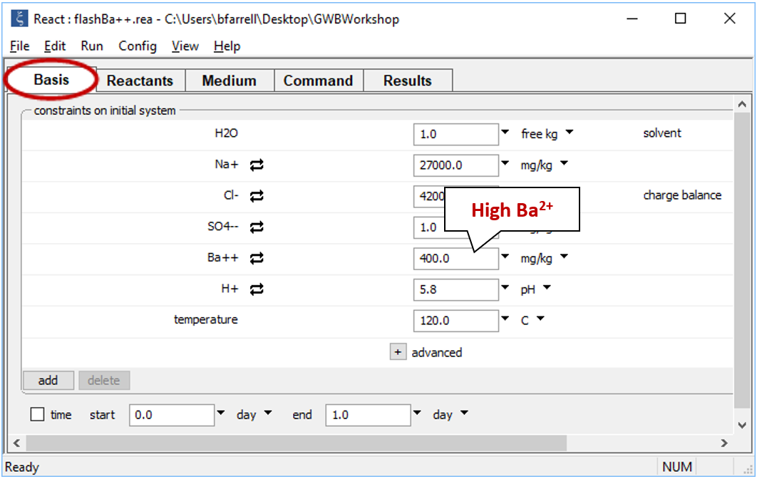
The pane shows concentrations of the dissolved components in the first fluid. The fluid is rich in Ba2+, but has a low SO42−concentration.
Equilibrate the fluid by selecting Run → Go. Next, select Run → Pickup → Reactants → Fluid. This “picks up” the result of our calculation and moves it to the Reactants pane
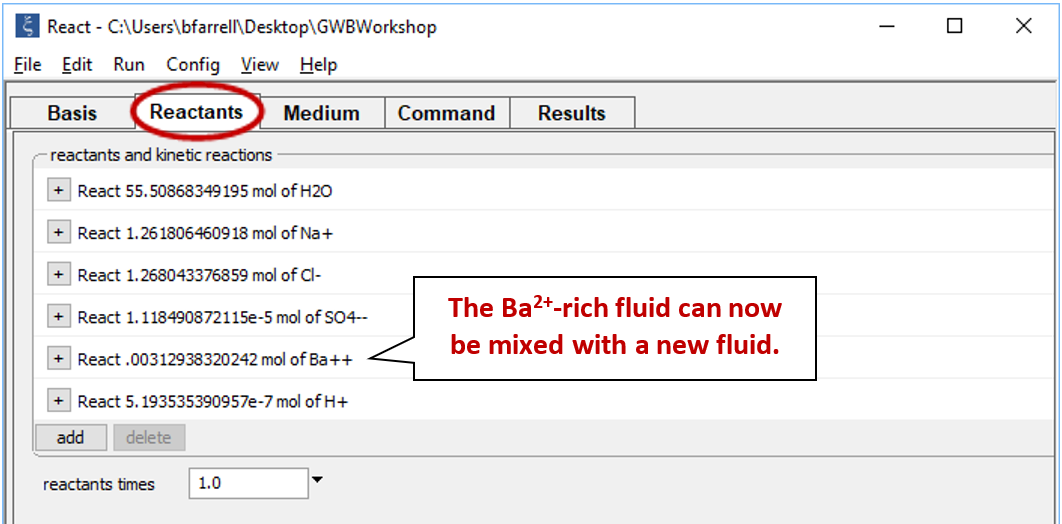
The first fluid is now a reactant that will mix into the second fluid.
Move back to the Basis pane, which is now empty, to set the composition of the second fluid. Drag file “flashSO4--.rea” into the pane. If a dialog box opens with the message “Reset configuration before reading script?”, be sure to click No

In contrast to the first fluid, the second contains little Ba2+, but is rich in SO42−.
On the Config → Stepping… dialog
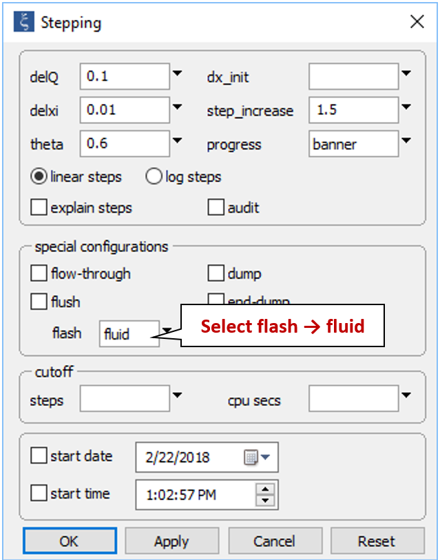
select the flash → fluid option and click OK. In a flash model, React removes the original fluid continuously as it adds the reactant fluid.
On the Config → Options… dialog, uncheck the “precipitation” option
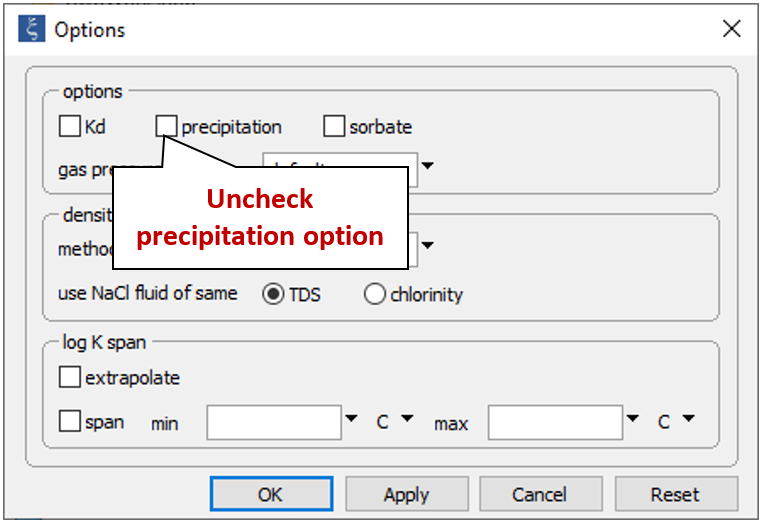
to prevent minerals from forming.
Select Run → Go. React will move to the Results pane and trace the simulation
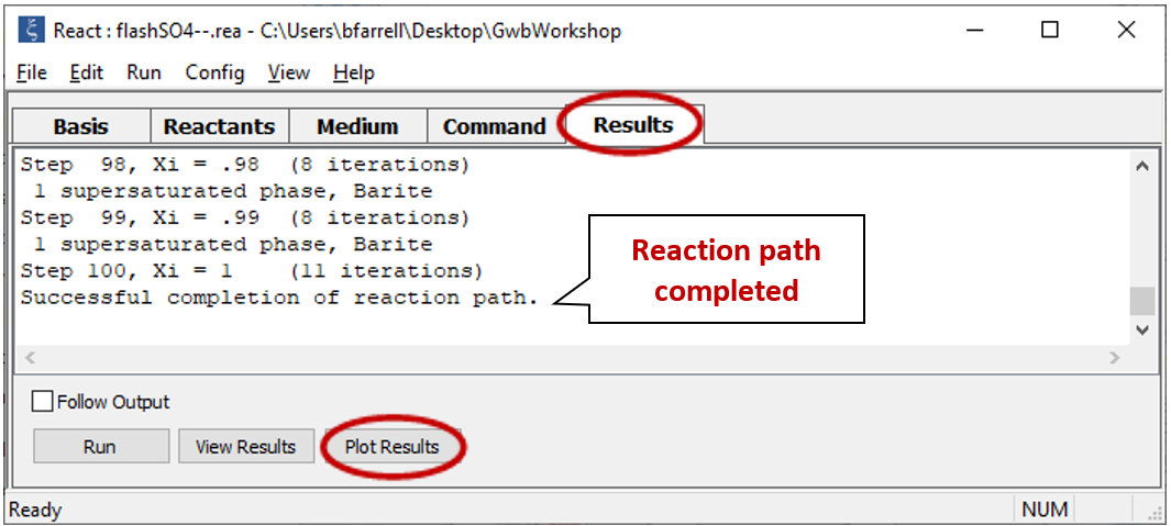
Click on  to launch Gtplot. Configure the plot as indicated below:
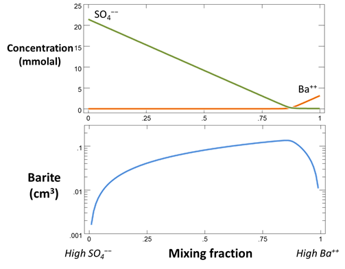
Now, make a flash diagram showing barite (BaSO4) saturation.
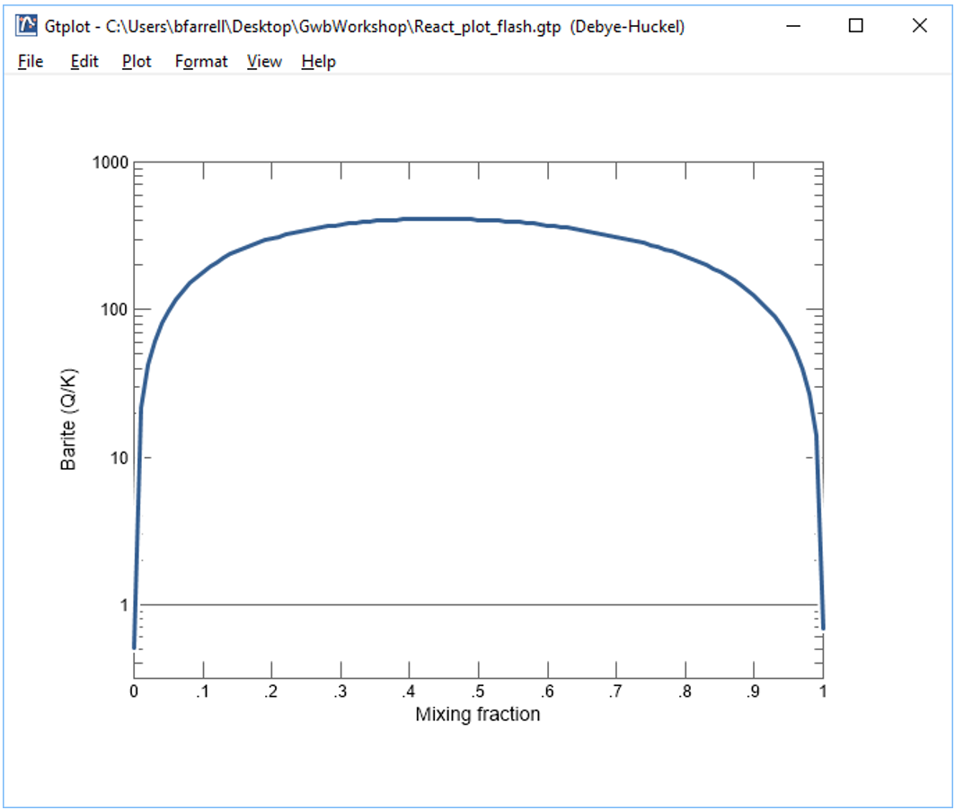
Is barite undersaturated or saturated in the mixed fluid?
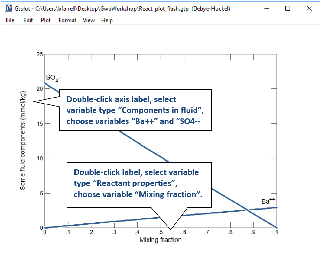
The horizontal axis shows the extent of mixing from purely the SO42− rich seawater fluid (composition set in the Basis pane) to purely the Ba2+ rich brine (composition set in the Reactants pane). A mixing value of 0.4, for example, represents a mixture of 60% of the original seawater and 40% of the reactant brine.
We plotted the concentration of the Ba++ and SO4−− components in the fluid and assembled the two plots into a single figure in MS PowerPoint.
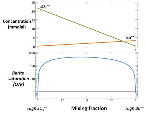
With no precipitation, the concentration of both components simply varies linearly with the mixing fraction. Looking at the saturation state of barite, the mineral is undersaturated in either end-member fluid, but becomes supersaturated in just about any mixing fraction
Return to the Config → Options… dialog and re-enable the “precipitation” option
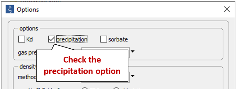
to create a model in which minerals can form; select Run → Go to recalculate the model.
Return to your plot of fluid composition. In what ways is the plot different from the run in which precipitation was not allowed?
Now plot mineral mass over the course of the mixing. What is the maximum amount of barite that precipitates as the fluids mix, in terms of mmol and cm3?
The added Ba++ reacts with SO4−− , which is in excess, to form barite. As a result, it does not accumulate in the mixture until the SO4−− becomes limiting. The SO4−− concentration decreases due to dilution and barite precipitation
Task 2: Sulfate scaling in North Sea oil fields
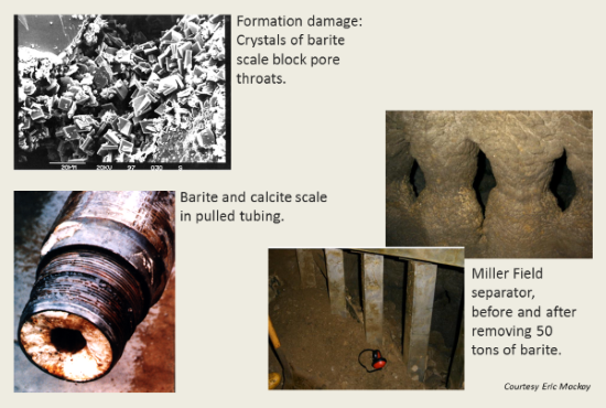
We now consider the offshore oil fields of the North Sea basin, where scaling in the formation and wellbore by sulfate minerals poses a considerable problem (e.g., Todd and Yuan, 1990, 1992; Yuan et al., 1994). Scaling occurs when seawater is used as a flooding or lifting agent during petroleum production.
Formation waters in the basin tend to be rich in barium and strontium but depleted in sulfate. Seawater, on the other hand, contains about 2700 mg/kg SO4−−. When the two fluids mix, the barium and strontium from the formation water react with seawater sulfate, forming minerals such as barite (BaSO4). The sulfate scale (commonly a solid solution of barite and celestite) plays havoc by reducing formation permeability and clogging the wellbore. Several examples of scaling from the North Sea oil fields are shown below
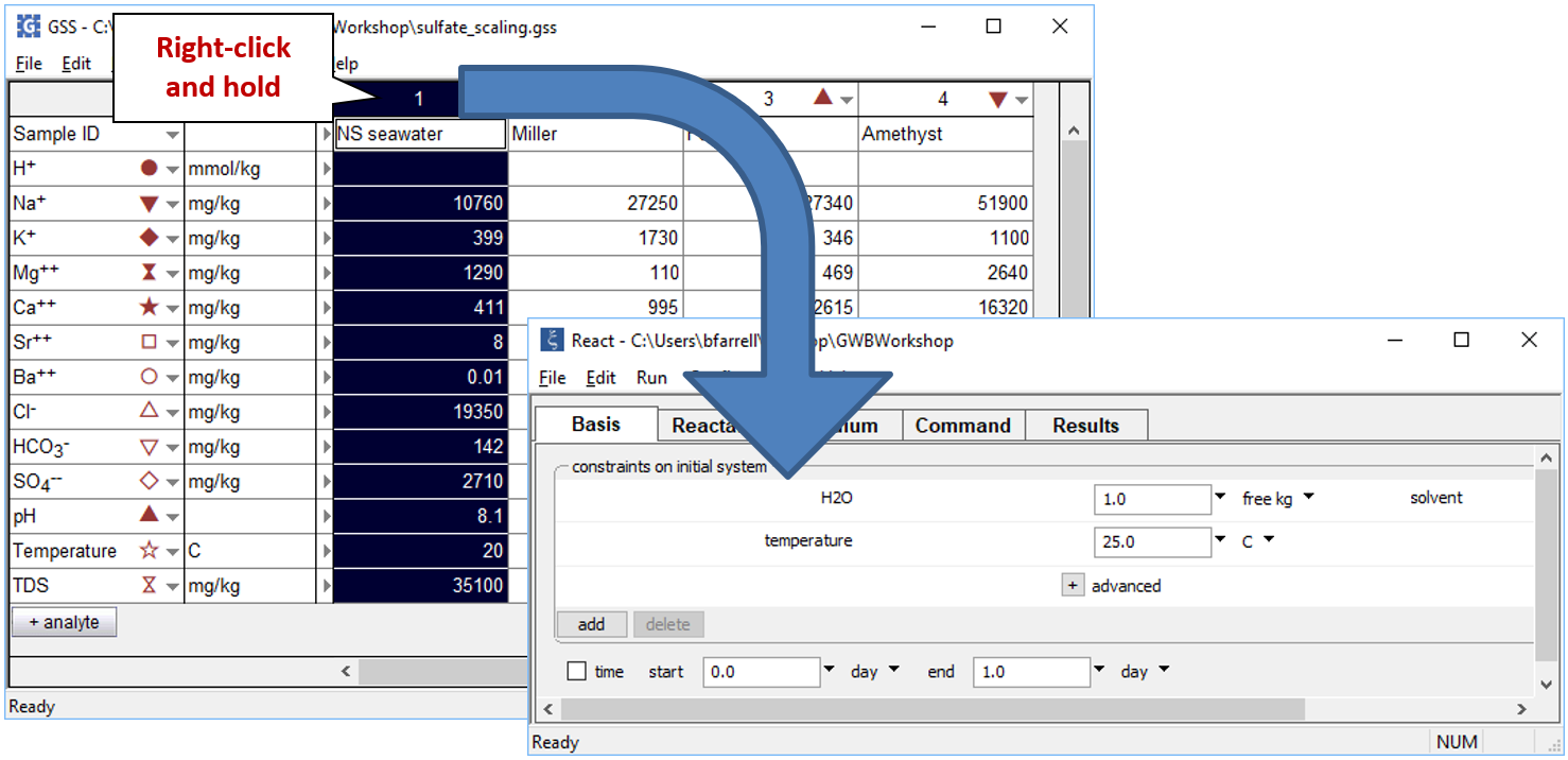
We'd like to evaluate the volume of scale that will precipitate from 1 kg of formation water as it mixes with seawater. To start, open the GSS file “sulfate_scaling.gss”, in which we've stored our analyses for the seawater (from Drever, 1988) and several formation waters from the North Sea
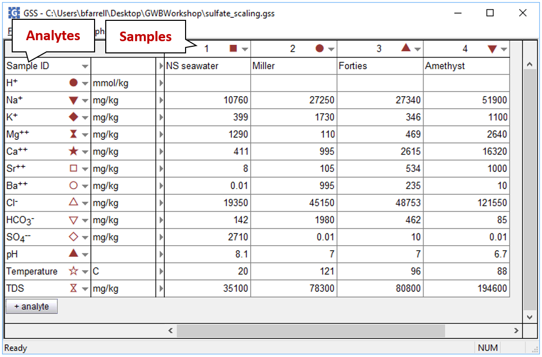
The file contains the complete analyses for each fluid.
To model the mixing process, we'll start by equilibrating the seawater sample and warming it to formation temperature. Open a new instance of React and move to the Basis pane. Now, right-drag (right-click and hold) the “NS_seawater” sample from the GSS file and drop it into React
Click the pulldown next to the unit for “temperature” and select the “sliding temperature” option. Set the “slide temperature to” field that appears to “121°C”, the formation temperature of the Miller fluid
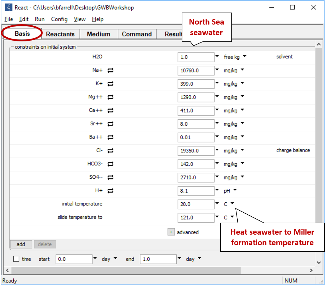
If you click the  button to expand the advanced option, you'll notice the value for TDS has been copied from the spreadsheet. This value is used for unit conversion within the program, but is not a constraint on the calculation.
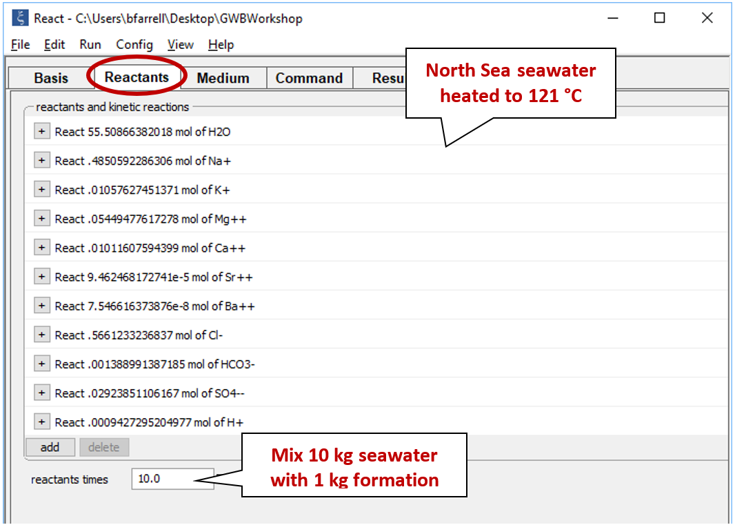
Select Run → Go to calculate the polythermal path. Now, pick up the resulting fluid to use as a reactant to mix into the Miller fluid. Click Run → Pickup → Reactants → Fluid.
Our heated seawater sample now appears on the Reactants pane. Enter a value of “10” next to the “reactants times” box to prescribe a mixing ratio of 10:1 parts seawater to formation fluid
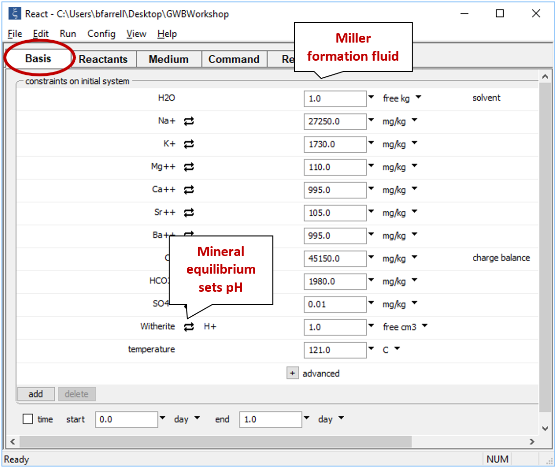
Move to the Basis pane and right-drag into it the Miller sample from the GSS datasheet. Remember to answer No if the program asks to reset. The Basis pane should look like this
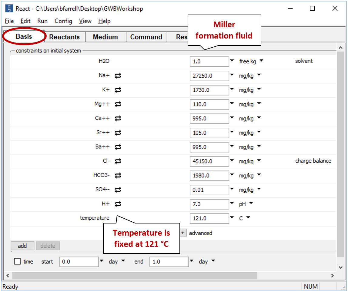
We've already heated the seawater to Miller formation temperature, so we leave “temperature” constant at its initial value of 121°C.
Since pH measurements from saline solutions are not reliable, we'll assume that pH is controlled by equilibrium with the most saturated carbonate mineral, which turns out to be witherite (BaCO3) or, for the Amethyst field, strontianite (SrCO3).
Click on the swap button next to the basis entry for "H+", select Mineral... → Witherite, and then set a nominal mass
From the Config → Stepping... dialog
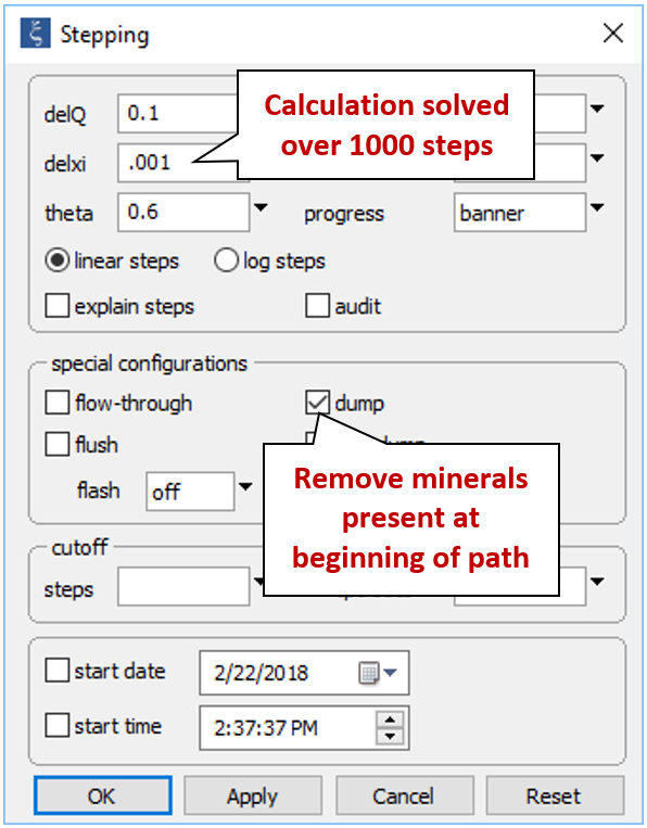
decrease the step size React will take to solve the simulation from “.01” to “.001”. Since we're only interested in the minerals that form as a result of mixing seawater with formation fluid, check the “dump” option, which will cause any minerals present at the start of the path (witherite, in this case) to be removed.
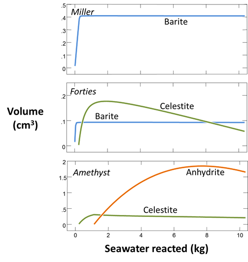
Set a suffix “_Miller_precip” and select Run → Go to calculate the mixing model. Plot the volumes of minerals that form as seawater reacts into the formation fluid.
Hint: the “Mass reacted, total” variable listed under “Reactant properties” includes every reactant added to the system. In this case, it's solvent water plus all of the solutes dissolved in seawater
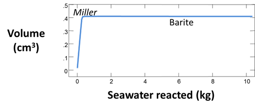
Barium in the Miller formation fluid reacts with the added sulfate from seawater to form barite. Once the barium concentration becomes limiting, precipitation ceases and the volume of barite holds steady.
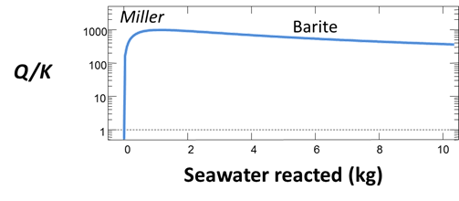
You can disable mineral precipitation like in Task 1 and repeat the mixing to calculate the saturation state of barite as seawater is mixed into the Miller formation fluid.
Barite is initially undersaturated in the sulfate-depleted Miller formation fluid, but as seawater is mixed in, it quickly becomes supersaturated. The saturation state decreases slightly as continued addition of seawater dilutes the barium in the mixture
If you'd like, you can reset React and repeat this procedure, this time mixing the Forties and Amethyst formation fluids with seawater. Do any other scale minerals form in these cases?
In the three simulations, the sulfate minerals form at mixing ratios related to their solubilities. Barite, the least soluble, forms early, when small amounts of seawater are added. The more soluble celestite forms only after the addition of somewhat larger quantities of seawater. Anhydrite, the most soluble of the minerals, forms from the Amethyst fluid at still higher ratios of seawater to formation fluid
Like before, the calculations were repeated after disabling mineral precipitation
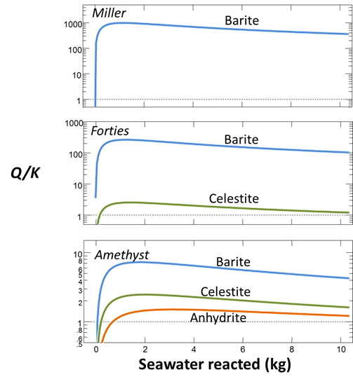
Comparing the volumes of scale produced in simulations in which minerals are allowed to form with the minerals' saturation states when precipitation is disabled, it is clear that no direct relationship exists between these values. In the Forties and Amethyst simulations, the saturation state of barite is greater than those of the other minerals that form, although the other minerals form in greater volumes. Whereas the Amethyst fluid is capable of producing about five times as much scale as fluids from the Miller and Forties fields, furthermore, the saturation states (Q/K) predicted for it are 1.5 to 2 orders of magnitude lower than for the other fluids.
Authors
Craig M. Bethke and Brian Farrell. © Copyright 2016–2026 Aqueous Solutions LLC. This lesson may be reproduced and modified freely to support any licensed use of The Geochemist's Workbench® software, provided that any derived materials acknowledge original authorship.
References
Bethke, C.M., 2022, Geochemical and Biogeochemical Reaction Modeling, 3rd ed. Cambridge University Press, New York, 520 pp.
Bethke, C.M., B. Farrell, and M. Sharifi, 2026, The Geochemist's Workbench®, Release 18: GWB Reaction Modeling Guide. Aqueous Solutions LLC, Champaign, IL, 219 pp.
Drever, J.I., 1988, The Geochemistry of Natural Waters, 2nd ed. Prentice-Hall, Englewood Cliffs, NJ.
Hutcheon, I., 1984, A review of artificial diagenesis during thermally enhanced recovery. In D.A. MacDonald and R.C. Surdam (eds.), Clastic Diagenesis. American Association of Petroleum Geologists, Tulsa, 413–429.
Todd, A.C. and M. Yuan, 1990, Barium and strontium sulphate solid-solution formation in relation to North Sea scaling problems. SPE Production Engineering 5, 279–285.
Todd, A.C. and M. Yuan, 1992, Barium and strontium sulphate solid-solution scale formation at elevated temperatures. SPE Production Engineering 7, 85–92.
Yuan, M., A.C. Todd and K.D. Sorbie, 1994, Sulphate scale precipitation arising from seawater injection, a prediction study. Marine and Petroleum Geology, 11, 24–30.
Comfortable with mixing and scaling?
You can also mix fluids stored in a GSS spreadsheet using the SmartMix wizard. Navigate to the Using GSS section to try it out for yourself.
Move on to the next topic, Introduction to Kinetics, or return to the GWB Online Academy home.