
Reaction kinetics
Reaction Kinetics is part of a free web series, GWB Online Academy, by Aqueous Solutions LLC.
What you need:
- GWB Standard recommended
-
Input files:
 KnQuartz.rea,
Redox.rea,
KnQuartz.rea,
Redox.rea,
 thermo_ladder.tdat,
Catalysis.rea
thermo_ladder.tdat,
Catalysis.rea
Download this unit to use in your courses:
- Lesson plan (.pdf)
- PowerPoint slides (.pptx)
Click on a file or right-click and select “Save link as…” to download.
Introduction
React, Phase2, X1t, and X2t can trace several types of reactions according to kinetic rate laws:
- Mineral precipitation and dissolution
- Redox transformations, including those associated with surfaces and enzymes
- Microbial metabolism and growth
- Formation and dissociation of aqueous and surface complexes
- Gas transfer
We'll start with the kinetics of mineral dissolution and precipitation. The time rate at which a mineral dissolves (positive rate) or precipitates (negative) can be described by a law:

(e.g., Lasaga, 1984). In this equation, AS is the surface area of the mineral, k+ is the intrinsic rate constant, and Q and K are the activity product and equilibrium constant for the dissolution reaction.
By this equation, a mineral will precipitate when it is supersaturated and dissolve when it is undersaturated at a rate that depends on its rate constant, which you supply, and surface area.
More complex rate laws, which account for the presence of species that promote or inhibit the rate of reaction, can also be considered. Consider the following examples of rate laws derived for albite dissolution:
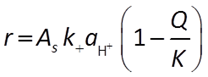
Where pH < 1.5, the activity of the H+ ion promotes the rate of reaction:
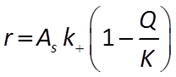
When pH is between 1.5 and 8, there are no promoting or inhibiting species:
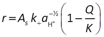
When pH > 8, the H+ is raised to a negative exponent, meaning it inhibits the rate of reaction. Another way to think about this is that the OH− promotes the rate of reaction:
The general form of the GWB's Built-in Rate Law for mineral dissolution and precipitation looks like this
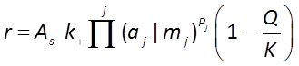
where r is the mineral's dissolution rate, AS is the surface area of the mineral, k+ is the intrinsic rate constant, aj, mj are the activity or concentration of promoting or inhibiting species, Pj is a species' power (+ is promoting, − is inhibiting), and Q and K are the activity product and equilibrium constant for the dissolution reaction.
The user supplies parameters for the rate law, including a specific surface area and rate constant for each mineral. The rate constant can be set directly or it can be calculated from the activation energy EA and pre-exponential factor A using the Arrhenius equation
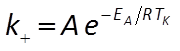
where R is the gas constant and TK is absolute temperature.
The Built-in Rate Law is sufficiently broad for most geochemistry applications, but the user can alternatively specify a custom rate law by writing an equation, BASIC script, or a compiled C++ function that the program can evaluate.
Task 1: Approach to equilibrium
Let's calculate how quartz sand reacts at 25°C with deionized water. How long will it take for a solution to come into equilibrium with silica sand? The reaction is Quartz → SiO2(aq).
According to Knauss and Wolery (1988), the above rate law is valid for neutral to acidic solutions; a distinct rate law applies in alkaline fluids, reflecting the dominance of a second reaction mechanism under conditions of high pH.
Double-click on file “KnQuartz.rea”, and when React opens, move to the Basis pane
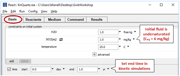
Here we've defined a dilute fluid, undersaturated with respect to quartz, and specified the time range of the calculation.
On the Reactants pane, note the kinetic rate law that governs the reaction of quartz
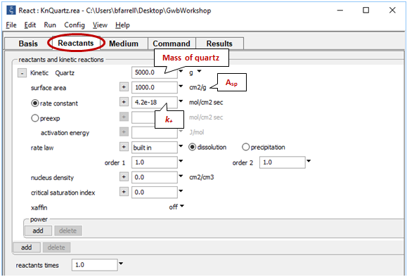
The rate constant k+ is from Rimstidt and Barnes (1980), and the specific surface area Asp is from Leamnson et al. (1969). React calculates the surface area of a mineral from its mass and the specific surface area in cm2 g-1 that you supply.
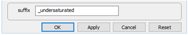
Note the suffix on the Config → Output… dialog
and select Run → Go. React will move to the Results pane and trace the simulation.
Before plotting the results, let's further test the case of a fluid supersaturated with respect to quartz. On the Basis pane, set an initial silica concentration of 12 mg kg-1

Next, open Config → Suppress… and suppress the silica polymorphs tridymite and chalcedony
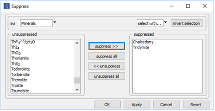
In this way, we keep our discussion simple by preventing those minerals from forming. On Config → Output..., set a suffix “_oversaturated” and repeat the run.
For each case, plot SiO2(aq) concentration and the fluid's saturation state versus time. How long does it take for the silica concentration to stabilize? Does the fluid approach equilibrium with quartz? Are laboratory experiments at this temperature likely to achieve equilibrium?
The results for both simulations, the undersaturated and supersaturated fluids, were plotted together using MS PowerPoint
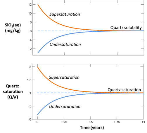
In the first simulation, the silica concentration gradually increases from the initial value, asymptotically approaching the equilibrium value of 6 mg kg-1 after about half a year of reaction.
In the second case, the supersaturated fluid, silica concentration gradually decreases from its initial value. As in the previous calculation, the fluid approaches equilibrium with quartz after about half a year.
Task 2: Redox kinetics—homogeneous catalysis
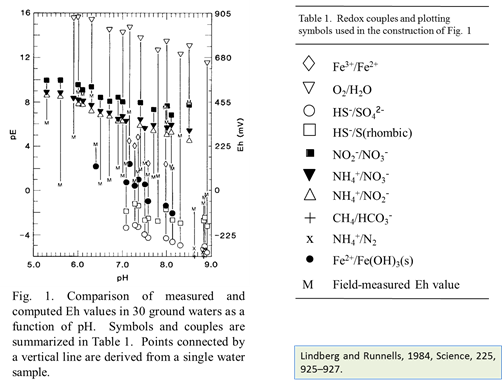
At low temperature, many redox reactions are unlikely to achieve equilibrium. Lindberg and Runnells (1984) demonstrated the generality of this problem. They compiled more than 600 water analyses that provided at least two measures of oxidation state and calculated species distributions for each sample. They then computed redox potentials for the various redox couples in the analysis, using the Nernst equation. Their results showed that redox couples in a sample generally failed to achieve equilibrium with each other.
Before this idea was widely accepted, the common approach in geochemical modeling was to assume that all redox reactions reached equilibrium. The user sets a single value for the system oxidation state, or a “Master Eh,” which controls the distribution of species among different oxidation states.
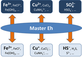
A more realistic approach is to allow for redox disequilibrium by disabling one or more redox coupling reactions. All coupled redox reactions still reflect the Master Eh for the system. Disabled redox couples, though, behave independently.
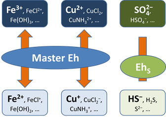
Any number of redox coupling reactions can be disabled. For any disabled pair, furthermore, a modeler can describe the rate at which mass in one oxidation state is transformed to another using a kinetic rate law.
When the reaction occurs entirely in solution, the process is termed homogeneous catalysis. A redox reaction of the form
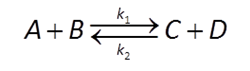
might be described by a rate law like
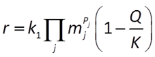
As an example, the oxidation of ferrous iron in the presence of oxygen

might be described by a rate law like this
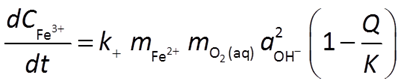
In this case, the ferrous iron ion, molecular oxygen, and the hydroxyl ion all promote the rate of the reaction. Because Fe2+ and O2(aq) are reactants, and because the reaction generates protons, the reaction will slow down as it moves forward.
With kinetic rate laws you can trace the progress over time of redox reactions as they move toward equilibrium. The following procedure models the oxidation of ferrous iron by molecular oxygen, assuming that the reaction produces ferric hydroxide.
Locate file “redox.rea” and double-click on it. When React opens, go to the Config → Redox Couples… dialog
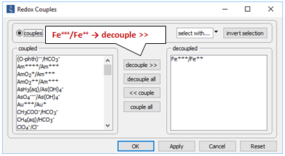
Here, the reaction between ferrous and ferric iron has been disabled. Iron in the simulation can therefore change redox state only by kinetic reaction.
The Basis pane
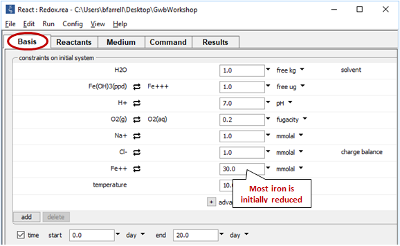
shows the fluid's initial composition. The ferrous and ferric components are constrained separately, since we've decoupled the Fe+++/Fe++ redox pair.
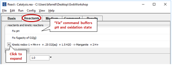
Move to the Reactants pane
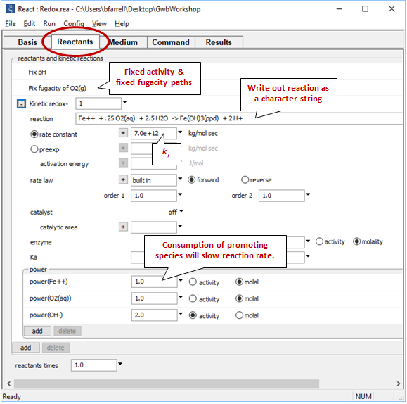
The “fix pH” and “fix fugacity of O2(g)” options simulate reaction in a pH-buffered laboratory experiment left open to oxygen in the atmosphere.
Click on the  button next to reactant “redox-1” to expand its entry. The reaction by which the ferrous iron component oxidizes has been written out explicitly as a character string that the program will read and interpret. If the kinetic reaction hadn't already been created, you would click here on add → Kinetic redox to do so.
To keep our discussion simple for the moment, we have suppressed the iron minerals goethite, hematite, and magnetite, each of which is more stable and slower to form than ferric hydroxide precipitate
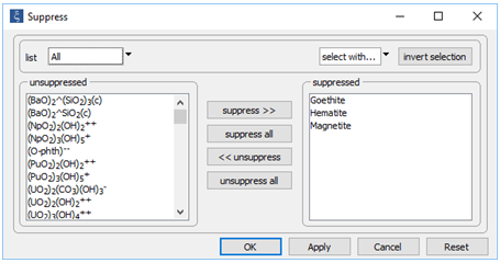
Note under Config → Output… the “_redox” suffix
Select Run → Go to calculate the model.
Plot how the Fe+++ and Fe++ components in the system vary with time. According to the form of the rate law, what is the order of the rate law? In our buffered system, what is the apparent order?
Here we've plotted the concentration of the thermodynamic components in the system (the sum of components in the fluid and in the “rock,” or minerals in our simulation) against time
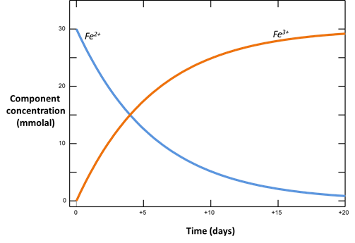
In our buffered system, the Fe2+ ion is the only promoting species whose concentration changes. Because it is set to a power of 1 in our rate law, the apparent order of the rate law is 1. As a result, the reaction rate is directly proportional to the concentration of the Fe2+ ion. As its concentration in solution decreases, the rate of the reaction slows.
Task 3: Redox kinetics—catalysis on mineral surfaces
Many redox transformation reactions occur on the surfaces of minerals. In that case, a redox reaction like

could be described by a rate law like

where AS is the catalyzing surface area.
You can choose a specific mineral as a catalyst (AS will be calculated from its mass), or set a total area. It is also possible to set parallel pathways for same redox reaction (i.e., the absence or presence of a catalyst). The total reaction rate would then be the sum of the rates.
Let's look at how mineral surfaces can promote redox reactions.
Double-click on file "catalysis.rea", and go to the Config → Redox Couples... dialog
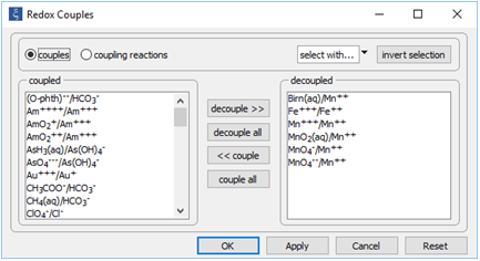
Note how we've disabled reaction between ferrous and ferric iron, as well as the reactions between several oxidation states of manganese. Iron and manganese in the simulation can change redox state only by kinetic reaction.
Click on File → View → .\thermo_ladder.tdat. This dataset is the “thermo.tdat” compilation we've been using, modified to allow decoupling of the Mn(III) and Mn(IV) redox states. Among other changes, the Mn+++ redox species has been imported from “thermo.com.v8.r6+.tdat”, and reactions for Mn(III) bearing minerals have been rebalanced in terms of the new redox species.
Look at the Basis pane

We consider a system containing reduced and oxidized manganese, as well as ferric hydroxide, which provides the catalyzing surface for manganese oxidation.
Move to the Reactants pane
We fix the pH and O2(g) fugacity to simulate a buffered experiment. Expand the entry for reactant “redox-1” to view the details of the kinetic rate law we've specified
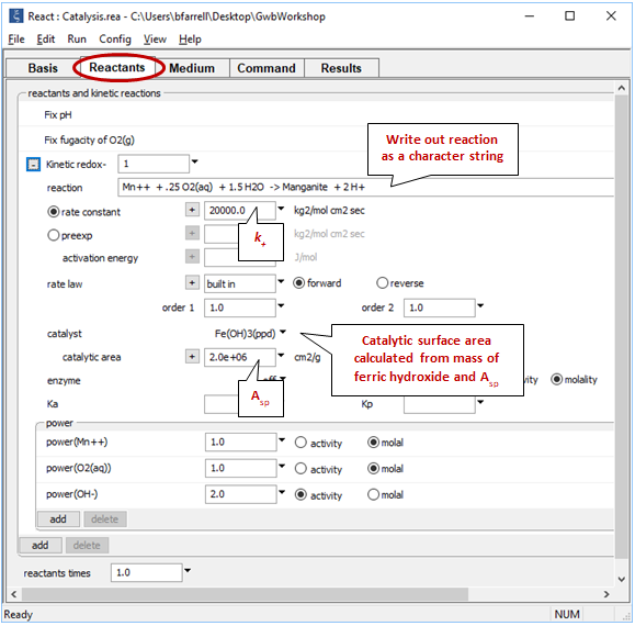
The oxidation of Mn++ to manganite (MnOOH) by molecular oxygen is catalyzed on the surface of ferric hydroxide.
On the Config → Suppress… dialog
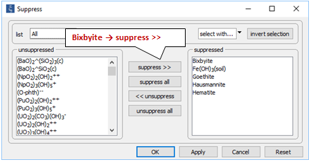
note the various iron and manganese minerals have been suppressed because they are stable, but unlikely to form over the time span of the simulation.
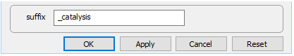
Note under Config → Output… the suffix "_catalysis"
Select Run → Go to trace the simulation.
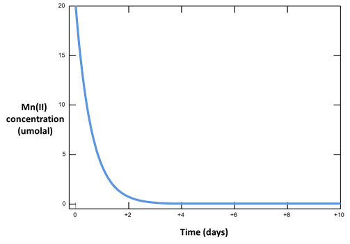
Plot versus time the concentration of the Mn++ component. How does it change, and why?
The rate of reaction is proportional to the catalyzing surface area, which remains constant, and the Mn2+ ion concentration, which is consumed as the reaction proceeds forward
Authors
Craig M. Bethke and Brian Farrell. © Copyright 2016–2026 Aqueous Solutions LLC. This lesson may be reproduced and modified freely to support any licensed use of The Geochemist's Workbench® software, provided that any derived materials acknowledge original authorship.
References
Bethke, C.M., 2022, Geochemical and Biogeochemical Reaction Modeling, 3rd ed. Cambridge University Press, New York, 520 pp.
Bethke, C.M., B. Farrell, and M. Sharifi, 2026, The Geochemist's Workbench®, Release 18: GWB Reaction Modeling Guide. Aqueous Solutions LLC, Champaign, IL, 219 pp.
Knauss, K.G. and T.J. Wolery, 1986, Dependence of albite dissolution kinetics on pH and time at 70 °C. Geochimica et Cosmochimica Acta 50, 2481–2497.
Knauss, K.G. and T.J. Wolery, 1988, The dissolution kinetics of quartz as a function of pH and time at 70 °C. Geochimica et Cosmochimica Acta 52, 43–53.
Lasaga, A.C., 1984, Chemical kinetics of water-rock interactions. Journal of Geophysical Research 89, 4009–4025.
Leamnson, R.N., J. Thomas, Jr. and H.P. Ehrlinger, III, 1969, A study of the surface areas of particulate microcrystalline silica and silica sand. Illinois State Geological Survey Circular 444, 12.
Lindberg, R.D. and D.D. Runnels, 1984, Groundwater redox reactions: an analysis of equilibrium state applied to Eh measurements and geochemical modeling. Science 225, 925–927.
Rimstidt, J.D. and H.L. Barnes, 1980, The kinetics of silica-water reactions. Geochimica et Cosmochimica Acta 44, 1683–1700.
Comfortable with reaction kinetics?
Move on to the next topic, Acid Drainage and Buffering, or return to the GWB Online Academy home.