
Hydrothermal fluids
Hydrothermal Fluids is part of a free web series, GWB Online Academy, by Aqueous Solutions LLC.
What you need:
- GWB Standard recommended
-
Input files:
 smokers_seawater.rea, smokers_hydrothermal.rea, thermophiles_hydrothermal.rea
Download this unit to use in your courses:
- Lesson plan (.pdf)
- PowerPoint slides (.pptx)
Click on a file or right-click and select “Save link as…” to download.
Introduction
Hydrothermal fluids, hot groundwaters that circulate within the Earth's crust, play central roles in many geologic processes, including the genesis of a broad variety of ore deposits, the chemical alteration of rocks and sediments, and the origin of hot springs and geothermal fields.
In the Spring of 1977, researchers on the submarine ALVIN discovered hot springs on the seafloor along the Galapogos spreading center. Later expeditions to the East Pacific Rise and Juan de Fuca spreading center found more springs, some discharging fluids as hot as 350°C. The hot springs are parts of large scale hydrothermal systems in which seawater descends into the oceanic crust, circulates near magma bodies where it warms and reacts extensively with deep rocks, and then under the influence of its buoyancy discharges back into the ocean.
Discovery of the hot springs has had an important impact in the geosciences, where geologists recognize the impact of the hydrothermal systems on controlling the thermal structure of the ocean crust and the composition of the oceans, as well as their role in producing ore deposits. A massive sulfide deposit, in fact, was found along the Galapagos spreading center. The springs also caused a stir in the field of biology because of the large number of previously unknown species such as tube worms discovered near the vents. Where the fluids discharge and mix with seawater, they cool quickly and precipitate clouds of fine-grained minerals. The clouds are commonly black with metal sulfides, giving rise to the term “black smokers”. Some vents give off clouds of white anhydrite; these are known as “white smokers”. The vents form structures where the hot fluids discharge. The structures can extend upward for some meters into the ocean, and are composed largely of anhydrite and sulfide minerals.
The chemical processes occurring within black smokers are certain to be complex because the hot, reducing hydrothermal fluid mixes so quickly with cool, oxidizing seawater that the mixture has little chance to approach equilibrium. Nonetheless, we'll attempt to construct a chemical model of the process.
Task 1: Black smokers
To model the mixing of a hydrothermal fluid with seawater at a vent, we equilibrate seawater at 4°C, pick up the fluid as a reactant, and then titrate it into a hot hydrothermal fluid.
Double-click on file “smokers_seawater.rea”. The Basis pane
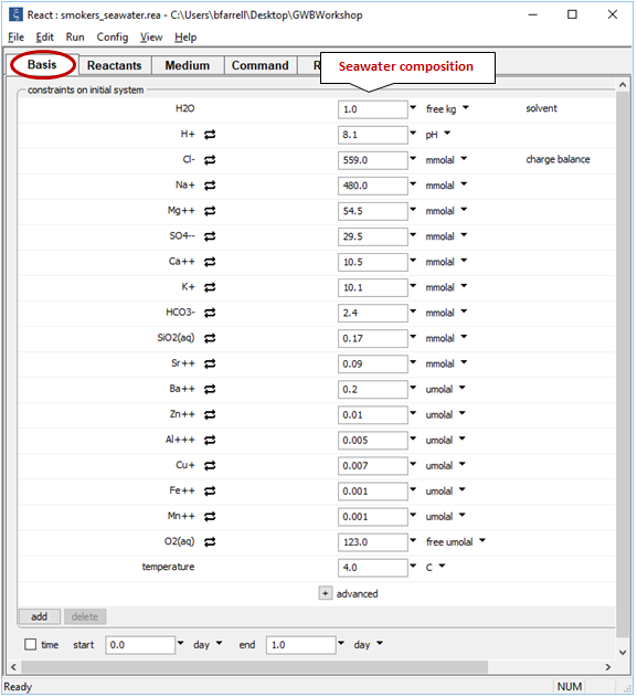
sets out the composition and temperature of deep seawater, the cold fluid in the simulation.
Equilibrate the seawater by going to Run → Go. Then, select Run → Pickup → Reactants → Fluid. This operation picks up the equilibrated seawater and moves it to the Reactants pane
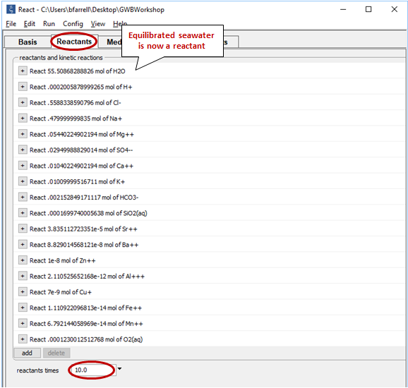
Set the value for the “reactants times” field at the bottom of the pane to “10”. This setting multiplies the extent of the reactant system tenfold. In this way we prescribe that seawater mix into the hydrothermal fluid up to a final ratio of 10:1.
Moving back to the (now empty) Basis pane, the next step is to define the hydrothermal fluid. Drag “smokers_hydrothermal.rea” from your course folder into React. If a dialog box with the message “Reset configuration before reading script?” opens, be sure to respond No
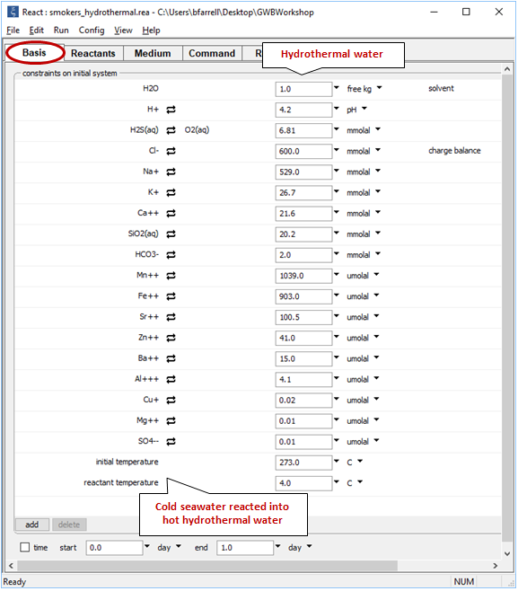
Note the initial temperature is taken from the input for the hydrothermal fluid, whereas the reactants have retained their temperature of 4°C. As cold fluid mixes into hot, temperature in the model will track the mixing ratio, accounting for the heat content of each fluid and the mixture's heat capacity.
Now, look at the Config → Suppress... dialog, where we have disallowed several minerals from forming
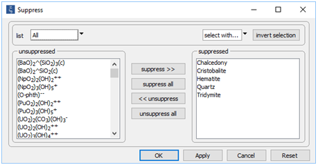
According to Mottl and McConachy (1990), amorphous silica (SiO2) is the only silica polymorph present in the “smoke” at the site. To allow it to form in the calculation, we suppress each of the more stable silica polymorphs. We also suppress hematite (Fe2O3) in order to give the iron oxy-hydroxide goethite (FeOOH) a chance to form.
On the Config → Stepping... dialog
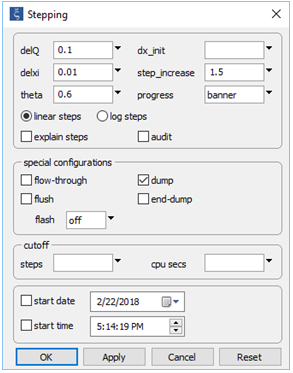
the “dump” option has been selected. This setting will cause the program to remove any minerals present in the initial system, before beginning to trace the reaction path.
Set a suffix “_smokers” and run the simulation

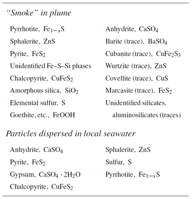
Plot against “Mass reacted, total” the minerals formed when the fluids mix. The table below shows minerals observed in samples taken above black smokers of the East Pacific Rise near 21°N (Mottl and McConachy, 1990)
How does the prediction compare to observation? Which minerals are observed but not predicted? Which minerals are predicted to form, but not observed? Why does anhydrite form and later begin to dissolve?
As shown in the figure below, anhydrite forms early on as calcium in the hydrothermal fluid reacts with sulfate in the seawater. Anhydrite begins to redissolve after a mixing ratio of about 1:1 as calcium becomes diluted in the mixture. After anhydrite, the most voluminous minerals to form are amorphous silica, talc [Mg3Si4O10(OH)2], and pyrite (FeS2)
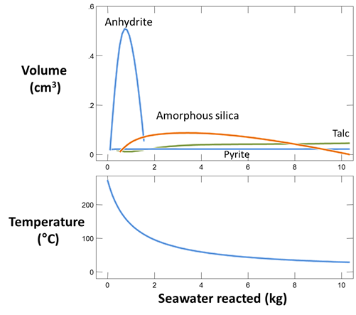
Amorphous silica forms because its solubility decreases at lower temperatures faster than it is diluted with seawater addition. Other minerals that form in small quantities include sphalerite (ZnS), barite (BaSO4), the zeolites mordenite (KAlSi5O12 · 3H2O) and clinoptilolite (CaAl2Si10O24 · 8H2O), and covellite (CuS). According to the data of Mottl and McConachy (1990), each of these minerals (lumping the talc and zeolites into the category of unidentified aluminosilicates) is observed suspended above the NGS vent. Even though the smoke at this site is described as black, sulfide minerals make up just a small fraction of the mineral volume precipitated over the course of the simulation.
A number of observed minerals do not form in the simulation. Wurtzite is metastable with respect to sphalerite, so it cannot be expected to appear in the calculation results. Similarly, the formation of pyrite in the simulation probably precludes the possibility of pyrrhotite precipitating. In the laboratory, and presumably in nature, pyrite forms slowly, allowing less stable iron sulfides to precipitate. Elemental sulfur at the site probably results from the incomplete oxidation of H2S, a process not accounted for in the simulation. There is no data in the LLNL database for marcasite or cubanite. Finally, goethite forms after we run the simulation to higher ratios of seawater to hydrothermal fluid than shown above.
Plot as well oxygen fugacity for the mixed fluid against “Mass reacted”. Has the fluid become oxidizing by the time it is ten parts seawater to one part hydrothermal fluid? Why or why not? Mottl and McConachy (1990) saw no evidence under the electron microscope that the sulfide minerals in the smoke were re-dissolving once they formed. Is this observation in agreement with the calculation?
The figure below shows the mixture's oxygen fugacity and the concentrations of several sulfur species as seawater is mixed into the hydrothermal fluid

Counterintuitively, the mixture remains reducing after the addition of oxygenated seawater to the reduced hydrothermal fluid. According to the reaction

and the composition of the two fluids, over 100 kg of seawater is needed to oxidize the H2S(aq) in the hydrothermal fluid. The decrease in oxygen fugacity results from the shift of the sulfide-sulfate buffer with temperature, which acts as long as any significant amount of H2S(aq) remains. The reducing conditions that are maintained throughout the mixing process help explain the lack of microscopic evidence of dissolution of the sampled sulfide minerals.
Task 2: Energy available to thermophiles
Subsea hydrothermal vents, as mentioned in the previous section, are sites of intense biological activity, relative to the rest of the ocean floor (e.g., Van Dover, 2000; Zierenberg et al., 2000). Life here ranges in complexity from single cells to higher forms such as tubeworms. The vent ecosystems are unique in many ways, including the fact that the primary producers create biomass not by photosynthesis, as is familiar in more accessible environments, but by chemosynthesis.
As fluid from the hydrothermal vent mixes with seawater, chemolithotrophic microbes harvest energy made available by chemical disequilibrium among redox reactions, forming the base of the ecosystem's food chain. Microbes can derive energy by converting CO2(aq) to methane using H2(aq) from the vent fluid, for example, or using the O2(aq) in seawater to oxidize H2S(aq).
We consider in this section the energy available to thermophilic microorganisms as a hydrothermal fluid mixes with seawater, following the work of McCollom and Shock (1997) and Jin and Bethke (2005), for a variety of such metabolisms. To model redox energetics during mixing, we follow the procedure in the previous section, but we disengage all redox couples except between O2(aq) and H2(aq). We assume the reaction

between these species proceeds spontaneously in the mixture.
Begin by reopening “smokers_seawater.rea”. When React starts, open the Config → Redox Couples... dialog
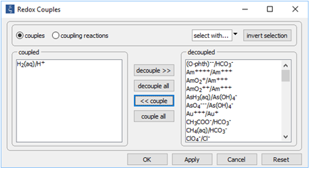
Click decouple all, then select the H2(aq)/H+ redox pair and click << couple. Click OK.
On the Basis pane
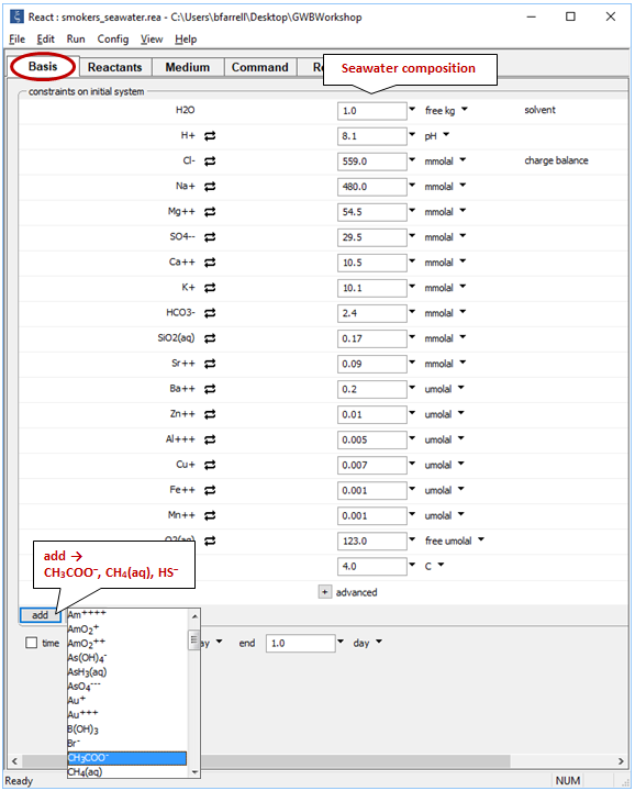
we need to expand composition to include small amounts of acetate, methane, and sulfide. Click  , then select one at a time the redox species from the pulldown menu
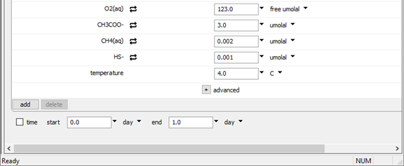
and set their constraints to 3 μmolal, .002 μmolal, and .001 μmolal, respectively, as shown above.
Equilibrate the seawater by clicking Run → Go and pick it up as a reactant with Run → Pickup → Reactants → Fluid
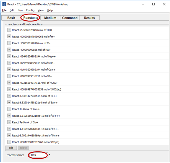
Set the “reactants times” field to 50 so the mixing ratio of seawater to hydrothermal fluid will extend as high as 50:1.
Drag file “thermophiles_hydrothermal.rea” from your course folder into the Basis pane. If asked “Reset configuration before reading script?”, be sure to click No.
This file is similar to “smokers_hydrothermal.rea”, from the previous task. In the file, however, each of the redox couples except H2-H+ has been disengaged. As well, acetate, methane, and sulfide components have been included. Finally, we've swapped H2(aq) in for O2(aq), and H2S(aq) in for HS−, since these species are more abundant in the reduced and low pH hydrothermal fluid.
Look at the bottom of the Basis pane to see the changes
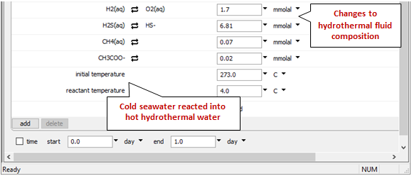
We've once again set up a polythermal path in which temperature depends on the proportion of hot and cold fluids in the mixture.
On the Config → Stepping... dialog
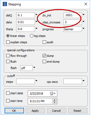
note we have set the dump option, as before. Instead of setting a constant step size, furthermore, we set a small initial step, but will allow the program to increase the length of reaction steps over the course of the run. In this way, we will create a detailed model of the initial stage of mixing.
On the Config → Output... dialog, note that we have set the value for dxplot to “0”. This causes the program to write the results for each step in the reaction path, so they are available for Gtplot to render

On this dialog, set a suffix “_thermophiles” and run the simulation.
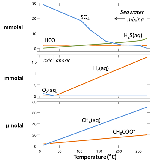
Plot against temperature the concentrations of the sulfate, sulfide, carbonate, methane, and acetate components, as well as the concentrations of the O2(aq) and H2(aq) species. What processes do you observe as the fluids mix?
During the mixing, concentrations of the sulfide, methane, and acetate components decrease as the vent fluid is diluted, and the sulfate concentration increases toward that of seawater. H2(aq) in the vent fluid attenuates not only by dilution, but by reaction with O2(aq). As the mixture reaches a temperature of about 38°C, the last of the H2(aq) in the anoxic fluid is oxidized in this way. Beyond this point, O2(aq) accumulates, leaving the mixture oxic. The temperature at which the transition from anoxic to oxic conditions occurs reflects the assumed supply of H2(aq) from the vent fluid, relative to O2(aq) from the seawater. If the vent produced a fluid poorer in dihydrogen, for example, or ambient seawater was more oxic, the transition would occur at a higher temperature
Plot against temperature the redox potentials of the various half-cell reactions. Which metabolisms appear to be favorable below 125°C, the approximate upper limit to microbial life, at temperatures where the mixed fluid is anoxic? Where the mixture is oxic?
As discussed in the redox disequilibrium lesson, the energy liberated by a redox reaction depends on the redox potential of the electron-donating half-cell reaction, relative to the electron-accepting reaction. In the calculation results, we can trace the redox potentials of half-cell reactions among sulfur species

and carbon species


as well as the hydrolysis reactions

and

as seawater is reacted into the hydrothermal vent fluid. The figure below shows the redox potentials of various half-cell reactions as a function of the temperature of the mixture
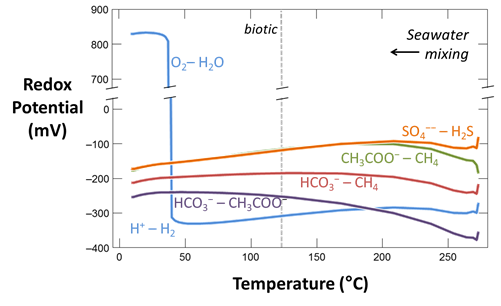
A redox reaction is favored thermodynamically when the redox potential for the electron-donating half-cell reaction falls below that of the accepting half-reaction. The redox potentials for the last two reactions listed, for electron acceptance by dioxygen and donation by dihydrogen, are equivalent in the model results, since we have set O2(aq) and H2(aq) to be in equilibrium.
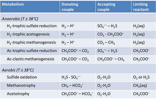
Taking the half-cell reactions in pairs, we can write a number of metabolisms by which microbes might derive energy during the mixing process. Several hydrogentrophic metabolisms are viable where the fluid mixture is anoxic: sulfate reduction

acetogenesis

and methanogenesis

Other possible anaerobic metabolisms are acetotrophic sulfate reduction

and acetoclastic methanogenesis

In each case, we write the metabolic reaction for the transfer of eight electrons, so the resulting energies can be compared on an equal basis.
Where the fluid is oxic, several aerobic metabolisms can proceed, including sulfide oxidation

methanotrophy

and homoacetotrophy

Reflecting the higher pH of the oxic relative to the anoxic fluid, we have written these reactions in terms of bicarbonate, rather than carbon dioxide. The table below summarizes the reactions described above.
The thermodynamic drive for each reaction is its negative free energy change, −ΔGr
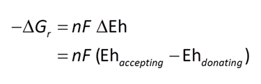
where ΔGr is the free energy change, in J mol−1 (or V C mol−1), n is the number of electrons transferred, and F is Faraday's constant, 96,485 C mol−1.
The figure below shows how the thermodynamic drive for each metabolism varies as the fluids mix, as determined from the calculated redox potentials. We consider only the mixing conditions where temperature falls below 150°C, somewhat higher than the maximum temperature at which microbial life has been observed
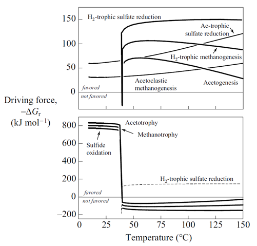
Each of the hydrogentrophic metabolisms is favored in the anoxic fluid, but cannot proceed once the mixture has become oxic, in the absence of dihydrogen. The other two anaerobic metabolisms, acetotrophic sulfate reduction and acetoclastic methanogenesis, do not depend on he presence of H2(aq) and are favored throughout the mixing.
The aerobic metabolisms—sulfide oxidation, methanotrophy, and acetotrophy—cannot proceed in the anoxic fluid, which is devoid of dioxygen, but are strongly favored in the oxic fluid. The thermodynamic drive for the aerobic processes under oxic conditions is about 800 kJ mol−1, much larger than the drives of less than about 150 kJ mol−1 observed under anoxic conditions for the anaerobic metabolisms.
The thermodynamic drives cited are the energy released instantaneously by the metabolic reaction, at the moment reaction commences. The drives tell whether the reaction can proceed, and whether it can supply enough energy for a cell to conserve energy by synthesizing ATP, as discussed in the lesson on microbial metabolism and growth. The values, however, do not describe how much energy microbes can extract from a fluid, and hence how much microbial growth the fluid can sustain.
The net amount of energy available from a fluid is its energy yield, given in units of energy per mass fluid, or J kg−1. The simplest way to caluculate the energy yield is to multiply the thermodynmamic drive by the mass of the limiting reactant, the reactant that will be first exhausted from the fluid as the reaction proceeds. We've included the limiting reactant for each metabolism in the table shown above.
The simplest way to calculate the energy yield is to multiply the thermodynamic drive by the mass of the limiting reactant, the reactant that will be first exhausted from the fluid as the reaction proceeds. The calculations, though, are approximate, because any reaction's thermodynamic drive diminishes as its reactants are consumed.
How does energy yield vary for the various metabolisms considered here? Does energy yield explain the microbial ecology observed at deep sea hydrothermal systems better than thermodynamic drive alone?
The figure below shows energy yields calculated as described above
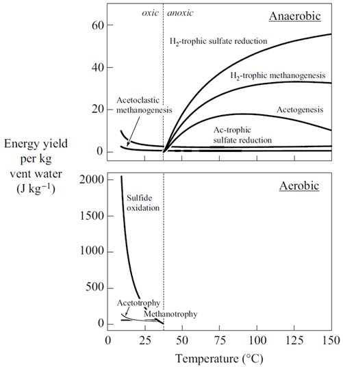
While the fluid remains anoxic, modest amounts of energy are available, most notably to hydrogentrophic sulfate reducers and hydrogentrophic methanogens. When the mixture turns oxic, however, much larger amounts of energy become available, primarily to the sulfide oxidizers. The total amount of energy that can be supplied to sulfide oxidizers during the mixing process dwarfs that available to all the other metabolisms combined.
The energetics depicted in this way are in accord with the microbial ecology observed at deep sea hydrothermal systems. Sediments and black smoker walls invaded by hydrothermal fluids there contain sparse microbial populations of mostly thermophilic methanogens and sulfate reducers. Abundant populations of mesophilic aerobes dominated by sulfide reducers, in contrast, are found in the open ocean where hydrothermal fluids mix freely with seawater.
Authors
Craig M. Bethke and Brian Farrell. © Copyright 2016–2026 Aqueous Solutions LLC. This lesson may be reproduced and modified freely to support any licensed use of The Geochemist's Workbench® software, provided that any derived materials acknowledge original authorship.
References
Bethke, C.M., 2022, Geochemical and Biogeochemical Reaction Modeling, 3rd ed. Cambridge University Press, New York, 520 pp.
Bethke, C.M., B. Farrell, and M. Sharifi, 2026, The Geochemist's Workbench®, Release 18: GWB Reaction Modeling Guide. Aqueous Solutions LLC, Champaign, IL, 219 pp.
Jin, Q. and C.M. Bethke, 2005, Predicting the rate of microbial respiration in geochemical environments. Geochimica et Cosmochimica Acta 69, 1133–1143.
McCollom , T.M. and E.L. Shock, 1997, Geochemical constraints on chemolithoautotrophic metabolism by microorganisms in seafloor hydrothermal systems. Geochimica et Cosmochimica Acta 61, 4375–4391.
Mottle, M.J. and T.F. McConachy, 1990, Chemical processes in buoyant hydrothermal plumes on the East Pacific Rise near 21°N. Geochimica et Cosmochimicha Acta 54, 1911–1927.
Van Dover, C.L., 2000, The Ecology of Deep-Sea Hydrothermal Vents. Princeton University Press.
Zierenberg, R.A., M.W.W. Adams and A.J. Arp, 2000, Life in extreme environments: Hydrothermal vents. Proceedings National Academy of Sciences 97, 12 961-12 962.
Comfortable with hydrothermal fluids?
Move on to the next topic, Phase Diagrams, or return to the GWB Online Academy home.