
Flow and transport
Flow and Transport is part of a free web series, ChemPlugin Modeling with Python, by Aqueous Solutions LLC.
What you need:
- ChemPlugin SDK 2025 recommended
-
Input file:
 FlowThrough1.py
Download this unit to use in your courses:
- Lesson Plan (.pdf)
- PowerPoint slides (.pptx)
Click on a file to open, or right-click and select “Save link as…” to download.
Introduction
Advective transport is the movement of chemical components among ChemPlugin instances, as the result of fluid flowing across links. To model advective transport, a client program must set the rate at which fluid crosses each link in a simulation, in terms of volume per unit time. The ChemPlugin instances on either side of a link, then, use that flow rate to figure fluxes across the link, in moles per unit time, of the chemical components considered in the simulation.
The advective flux Jio of chemical component i, in mol s−1, is given
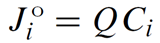
where Q is the flow rate across a link in m3 s−1 and Ci is the concentration of i, in mol m−3.
The transport law is set out in terms of the concentration itself, rather than a derivative. As such, advective transport is commonly referred to as a zero-order process; hence, the notation. First-order transport, in which the transport law is written in terms of the gradient (i.e., the first-order derivative) of concentration, is treated later.
A client uses the “FlowRate()” member function to specify the fluid volume crossing a link per unit time
     # Flow from cp1 to cp0
    cp0, cp1 = ChemPlugin(), ChemPlugin()
    link = cp0.Link(cp1)
    link.FlowRate(0.5e6, "cm3/s")
        or
    link.FlowRate(0.5)  # default unit = m3/s
Flow is by convention positive when it moves toward the instance that created the link, and negative in the opposite direction.
The “FlowRate()” member function can also be used to retrieve the rate of flow across a link, as previously set
    flow = link.FlowRate("cm3/s")
        or
    flow = link.FlowRate()  # unit = m3/s
In a typical client program, the time marching loop is the outer loop. Within the time marching loop, there may be loops over the instances that make up the domain. Use the “AdvanceTransport()” member function to trigger an instance to move mass into or out of an instance. The function evaluates the effect of mass transport on the instance's chemical composition over the course of the current time step.
For steady flow, call the “FlowRate()” member function once, before entering the time marching loop. For transient flow, alternatively, call “FlowRate()” at the head of each pass through the loop.
As an example of how a client program can use linked ChemPlugin instances to model reaction processes in open systems, we construct here a client program that simulates a well-stirred flow-through reactor.

In our program, a ChemPlugin instance “cp_inlet” represents the inlet fluid that passes into the well-stirred reactor, which is represented by instance “cp”. Fluid from “cp_inlet” flows across a link into “cp”, displacing fluid from it. The displaced fluid follows an open link to the free outlet, where it is lost.
To get started, right-click on FlowThrough1.py and open it in Notepad++.
To begin, the client sets a ChemPlugin instance “cp_inlet” to represent the inlet fluid, which is a dominantly HCl solution of pH 1
    from ChemPlugin import *

    print("Model a flow-through reactor\n")

    # Configure and initialize the inlet fluid.
    cp_inlet = ChemPlugin("stdout")
    cmds = "Ca++ = 1 mmol/lg; HCO3- = 1 mmol/kg; pH = 1; balance on Cl-"
    cp_inlet.Config(cmds)
    cp_inlet.Initialize()
The client creates the instance, setting it to write out console messages, configures it according to the character string pointed to by “cmds”, and initializes it.
The inlet instance serves in the program as a static fluid of known composition. There is no need to specify a time span for the instance, nor does the instance's extent (i.e., it's volume or mass) need to be known; by the zero-order equation above, the concentrations but not the masses of the fluid's chemical components enter into the transport calculation.
Next, the client sets a ChemPlugin instance “cp” to act in the simulation as a stirred reactor.
    # Configure and initialize the stirred reactor.
    cp = ChemPlugin("stdout")
    cmds = ("swap Calcite for Ca++", "Calcite = 0.03 free m3", "Cl- = 1 mmol/kg",
            "swap CO2(g) for H+", "fugacity CO2(g) = 1", "balance on HCO3-",
            "volume = 1 m3", "fix f CO2(g)", "delxi = 0.01", "pluses = banner")

    for c in cmds: cp.Config(c)
    cp.Initialize(1.0, "day")
The client configures the instance to contain a fluid in equilibrium with CaCO3 and a CO2 reservoir of known fugacity, which is held constant over the simulation. The instance volume is set to 1 m3, of which 0.03 m3 consists of CaCO3.
Setting “delxi” to 0.01 prescribes the simulation traverse 100 time steps over the course of the simulation, which is set to span 1 day. The command “pluses = banner” sets the instance to write a banner-style output at each reaction step.
We next link instance “cp” to instance “cp_inlet”, create an open link from “cp”, and set a flow rate across each link.
    # Link reactor to inlet and free outlet; set rate of flow.
    link1 = cp.Link(cp_inlet)
    link2 = cp.Link()

    link1.FlowRate(10.0, "m3/day")
    link2.FlowRate(-10.0, "m3/day")
Since the flow rate is 10 m3 day−1 and the simulation spans 1 day, 10 m3 of fluid will pass into “cp”, and an equivalent volume will be displaced across the free outlet.
Note especially that the flow rate across the first link, from “cp” to “cp_inlet”, is positive, since the fluid is flowing toward “cp”. The rate at which fluid is displaced across the second link, the free outlet, on the other hand, is negative, since the flow is in this case away from “cp”.
The time marching loop is similar to the loop we constructed in the titration model, except we have added a call to member function “AdvanceTransport()”:
    cp.PlotHeader("FlowThrough.gtp")
    cp.PlotBlock()

    # Time marching loop.
    while True:
        deltat = cp.ReportTimeStep()
        if cp.AdvanceTimeStep(deltat): break
        if cp.AdvanceTransport(): break
        if cp.AdvanceChemical(): break
        cp.PlotBlock()

    input("Done!")
By calling “AdvanceTransport()”, we trigger instance “cp” to account for how flow from “cp_inlet” into “cp”, as well as flow from “cp” into the free outlet, affect the chemical composition of the reactor.
Note that we've used calls to member functions “PlotHeader()” and “PlotBlock()” to trigger “cp” to create a plot output file, “FlowThrough.gtp”.
Task 1: Running a flow-through reactor model
Double-click on “FlowThrough1.py” to run the client program, which produces the following on the console window:
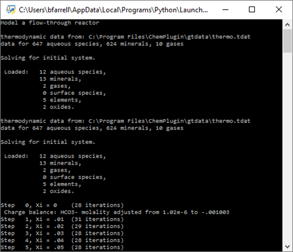
Two ChemPlugin instances, representing the inlet and the stirred reactor, are initialized, and then the client traces reaction within the stirred reactor.
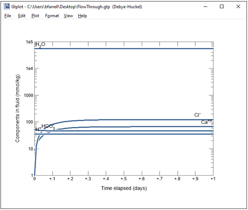
Double-click the “FlowThrough.gtp” dataset that's generated to render the calculation results graphically with program Gtplot.
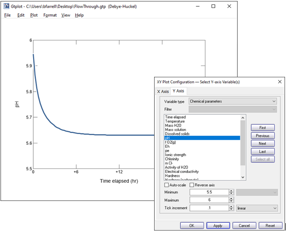
Double click on the x axis label and select “hr” for the units, then uncheck “Auto-scale” and set the “Maximum” to 24, with a “Tick Increment” of 6.
On the Y Axis pane choose “Chemical parameters” and select pH. Uncheck “Auto-scale” and set the “Minimum” to 5.5, “Maximum” to 6, and “Tick Increment” to 0.1.
Change the y axis variable type to “Components in fluid” and select Ca++ and HCO3-. Choose “mmol/kg” for the units and set a linear scale.
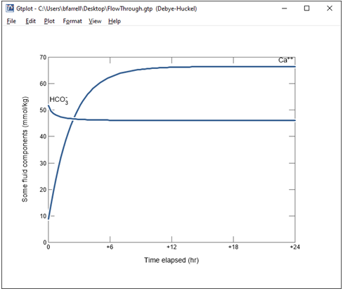
What controls the concentration of calcium and carbon in solution?
Finally, change the y axis variable type to “Minerals” and select Calcite. Choose “mmol/kg” for the units and set a linear scale.
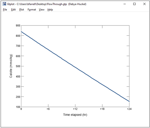
Together with the fugacity buffer, the presence of calcite in the reactor buffers solution composition.
What will happen if the calcite buffer is completely exhausted?
Authors
Craig M. Bethke and Brian Farrell. © Copyright 2016–2026 Aqueous Solutions LLC. This lesson may be reproduced and modified freely to support any licensed use of The Geochemist's Workbench® software, provided that any derived materials acknowledge original authorship.
References
Bethke, C.M., 2022, Geochemical and Biogeochemical Reaction Modeling, 3rd ed. Cambridge University Press, New York, 520 pp.
Bethke, C.M., 2026, The Geochemist's Workbench®, Release 18: ChemPlugin™ User's Guide. Aqueous Solutions LLC, Champaign, IL, 303 pp.
Carslaw, H.S. and Jaeger, J.C., 1959, Conduction of Heat in Solids. Clarendon Press, Oxford, 510 pp.
Comfortable with Flow and Transport?
Move on to the next topic, Diffusion and Dispersion, or return to the ChemPlugin Modeling with Python home.