
Diffusion and dispersion
Diffusion and Dispersion is part of a free web series, ChemPlugin Modeling with Python, by Aqueous Solutions LLC.
What you need:
- ChemPlugin SDK 2025 recommended
-
Input file:
 Diffusion1.py
Download this unit to use in your courses:
- Lesson Plan (.pdf)
- PowerPoint slides (.pptx)
Click on a file to open, or right-click and select “Save link as…” to download.
Introduction
Dispersive (or diffusive) mass flux is the net rate chemical mass moves in response to a concentration gradient, as given by Fick's law
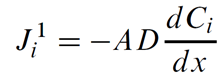
In this equation, Ji1 is the flux of chemical component i in mol s−1, A is the link's cross-sectional area in m2, D is the Fickian coefficient in m2 s−1, and Ci is the concentration of component i in mol m−3. The notation Ji1 reflects the first-order derivative in the transport law.
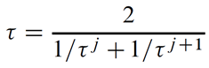
ChemPlugin instances employ a transmissivity τ, in units of m3 s−1, to calculate first-order fluxes in discrete domains
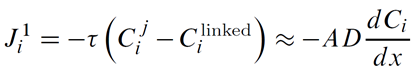
Here Cij and Cilinked are the concentrations of component i at the originating and linked instances, respectively.
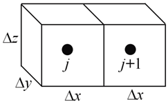
For a homogeneous medium and uniform grid
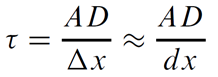
In the general case, instances may vary in D and spacing Δx
The overall transmissivity is given as the harmonic mean of τ at the two instances
which works out to
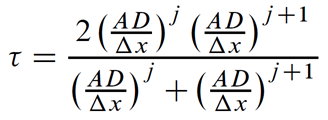
for the heterogeneous, arbitrarily gridded case.
A client uses member function “Transmissivity()” to set transmissivity across a link
    cp0, cp1 = ChemPlugin(), ChemPlugin()
    link = cp0.Link(cp1)
    link.Transmissivity(2.e3, "cm3/s")
        or
    link.Transmissivity(2.e-3)  # default unit = m3/s
The unit field may be any unit of flow rate as set out in the Units Recognized appendix to the ChemPlugin User's Guide. If the client does not specify a second argument, the value is taken to be in m3 s−1.
When the “Transmissivity()” member function is called without an argument, it returns the transmissivity currently set for a link. The examples below
    trans = link.Transmissivity("cm3/s")
        or
    trans = link.Transmissivity()  # in m3/s
store the current transmissivity value across “link” in variable “trans”, in units of cm3 s−1 or the default m3 s−1.
Task 1: Diffusion model
As a demonstration of how a client program can use ChemPlugin to model diffusive transport, we construct here a one-dimensional model of diffusion within a porous medium. In our model, the domain is 100 cm long and contains a NaCl solution of concentration 1 mmol/kg where 0 < x < 50 cm, and 0.001 mmol/kg where 50 < x < 100 cm. At t = 0, the salt begins diffusing from left to right, toward large x.
To get started, right-click on Diffusion1.py and open it in Notepad++.
The purpose of function “write_line()” is to write the simulation results to a file at specific points in time, instead of writing output after each time step, which would be unwieldy. The code is:
    from ChemPlugin import *
    import sys

    def write_line(f, cp, gap, then):
        now = cp[0].Report1("Time", "years")
        if (then - now) <= gap / 1e4:
            f.write("%8.4f" % now)
            for c in cp:
                f.write("\t%8.4f" % c.Report1("concentration Na+", "mmol/kg"))
            f.write("\n")
            f.flush()
            then += gap
        return then

    def end_run(code):
        input("Done!")
        sys.exit(code)

    print("Model diffusion in one dimension\n")
Here, “f” is a reference to the output stream, “cp” is the origin of a vector of “nx” references to ChemPlugin instances, “gap” is the separation in years between output points, and “then” is a reference to a memory location in the calling program. The memory location holds the time level, in years, at which the next output event is to occur.
The simulation parameters are the numerical values that define the transport model.
    # Simulation Parameters
    nx = 100                     # number of instances along x
    length = 100.0               # cm
    deltax = length / nx         # cm
    deltay = 1.0                 # cm
    deltaz = 1.0                 # cm
    porosity = 0.25              # volume fraction
    diffcoef = 1e-6              # cm2/s
    xstable = 0.9                # unitless
    time_end = 15.0              # years
    delta_years = time_end / 3.  # years
    next_output = 0.0            # years
Here, we note the length “deltax” of the instances is the domain size “length” divided by the number “nx” of ChemPlugin instances carried.
The transmissivity “trans” is the product of the cross-sectional area “deltay * deltaz”, the porosity, and the diffusion coefficient “diffcoef”, divided by “deltax”.
Variable “xstable” holds the stability factor Xstable, and “time_end” is the duration of the simulation. The value set for “delta_years” is the gap between the output events, and “next_output” is the time level at which the next event is to be triggered.
The next block of code opens an output stream to a disk file and writes a line identifying the position along x at which each ChemPlugin instance will be positioned.
    # Open output file and write instance positions on the first line
    f = open("Diffusion.txt", "w")
    f.write("   years")
    for i in range(nx):
        f.write("\t%8.4f" % ((i + 0.5) * deltax))
    f.write("\n")
Next, the client program sets out to create, configure, and initialize each ChemPlugin instance to make up the domain.
    # Configure and initialize the instances
    cmd0 =  "volume = " + str(deltax * deltay * deltaz) + " cm3; "
    cmd0 += "porosity = " + str(porosity) + "; "
    cmd0 += "time end = " + str(time_end) + " years; "
    cmd0 += "Xstable = " + str(xstable)

    cmd1 = "Na+ = 1 mmol/kg; Cl- = 1 mmol/kg"
    cmd2 = "Na+ = 0.001 mmol/kg; Cl- = 0.001 mmol/kg"

    cp = [ChemPlugin() for i in range(nx)]
    cp[0].Console("stdout")
    cp[0].Config("pluses = banner")

    for i in range(nx):
        cp[i].Config(cmd0)
        if i < nx / 2:
            cp[i].Config(cmd1)
        else:
            cp[i].Config(cmd2)

        if cp[i].Initialize():
            print("Instance " + str(i) + " failed to initialize")
            end_run(-1)

    next_output = write_line(f, cp, delta_years, next_output)
The first lines of the code set three character strings to hold ChemPlugin configuration commands: “cmd0”, “cmd1”, and “cmd2”. The former, “cmd0”, is to be applied to each of the instances, whereas “cmd1” pertains to instances on the left side of the domain, and “cmd2” to only the right-side instances.
The client next instantiates a vector of “nx” instances, but sets only the first to write console out messages, using the “banner” format to trace time stepping. If each of the instances had been set to produce console output, the result would be overwhelming and largely redundant. Finally, the client enters a loop in which it configures each ChemPlugin instance in the domain, and initializes it. If any of the instances does not initialize, the client exits with a non-zero status code.
The loop for linking the instances into a one-dimensional chain and setting transmissivity for each link is:
    # Link the instances
    trans = deltay * deltaz * porosity * diffcoef / deltax
    for i in range(1, nx):
        link = cp[i].Link(cp[i - 1])
        link.Transmissivity(trans, "cm3/s")
The loop starts by linking the second instance (index 1) to the first (index 0), then links the third to the second, and so on. For each link, the client sets the corresponding transmissivity, as previously stored in “trans”.
Note the best practice of linking an instance to the instance behind it, rather than in front of it. Flow across a link in ChemPlugin is positive when it moves toward the instance that originated the link, away from the linked instance. By the convention of linking backwards, then, flow is positive toward instances of increasing index.
The time marching loop begins each pass by querying the instances for the preferred time step, as determined honoring the stability considerations outlined above. Then, taking the minimum of the steps reported, it steps forward in time, advances the transport equations, and advances the chemical equations. Finally, it passes the results to “write_line()” and returns to make another step.
    # Time marching loop
    while True:
        deltat = 1e99
        for c in cp:
            deltat = min(deltat, c.ReportTimeStep())
        for c in cp:
            if c.AdvanceTimeStep(deltat): end_run(0)
        for c in cp:
            if c.AdvanceTransport(): end_run(-1)
        for c in cp:
            if c.AdvanceChemical(): end_run(-1)

        next_output = write_line(f, cp, delta_years, next_output)
Running the client produces the following
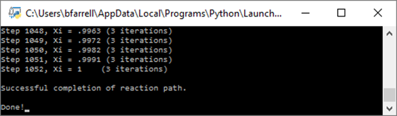
on the console window
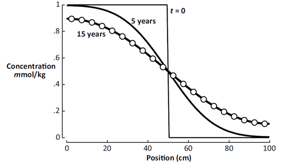
Once the run is complete, open the “Diffusion.txt” file that's generated by the client in a program such as MS Excel.
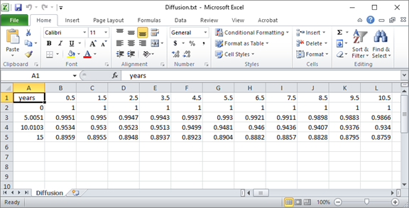
You can quickly plot the salinity profile across the domain at various points in the simulation.
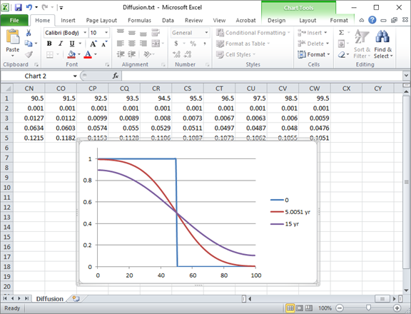
The plot below shows the calculation results after 5 years and 15 years.
The circles in the diagram correspond to the analytic solution to the diffusion equation at t = 15 years, from Carslaw and Jaeger's 1959 text, demonstrating correctness of the client's results.
Authors
Craig M. Bethke and Brian Farrell. © Copyright 2016–2026 Aqueous Solutions LLC. This lesson may be reproduced and modified freely to support any licensed use of The Geochemist's Workbench® software, provided that any derived materials acknowledge original authorship.
References
Bethke, C.M., 2022, Geochemical and Biogeochemical Reaction Modeling, 3rd ed. Cambridge University Press, New York, 520 pp.
Bethke, C.M., 2026, The Geochemist's Workbench®, Release 18: ChemPlugin™ User's Guide. Aqueous Solutions LLC, Champaign, IL, 303 pp.
Carslaw, H.S. and Jaeger, J.C., 1959, Conduction of Heat in Solids. Clarendon Press, Oxford, 510 pp.
Comfortable with Diffusion and Dispersion?
Move on to the next topic, Heat Transfer, or return to the ChemPlugin Modeling with Python home.