
Geochemical buffers
Geochemical Buffers is part of a free web series, GWB Online Academy, by Aqueous Solutions LLC.
What you need:
- GWB Standard recommended
-
Input files:
 buffers.rea,
mineral_buffers.rea,
buffers.rea,
mineral_buffers.rea,
 Fe_trace.ac2, fugacity_buffers.rea
Download this unit to use in your courses:
- Lesson plan (.pdf)
- PowerPoint slides (.pptx)
Click on a file or right-click and select “Save link as…” to download.
Introduction
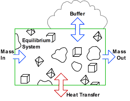
The heart of a geochemical model is the equilibrium system, which contains an aqueous fluid and, optionally, one or more minerals. The system's constituents remain in chemical equilibrium throughout the calculation. Transfer of mass into or out of the system and variation in temperature drive the system to a series of new equilibria over the course of the reaction path.
In this section, we consider how to construct reaction paths that account for the effects of simple reactants, a name given to reactants that are added to or removed from a system at constant rates. We commonly refer to such a path as a titration model, because at each step in the process, much like in a laboratory titration, the model adds an aliquot of reactant mass to the system.
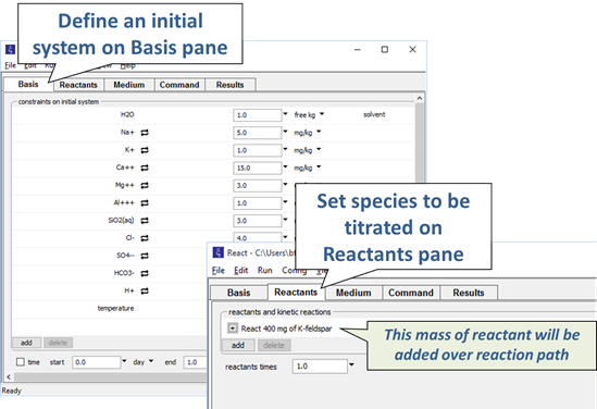
As an example, we could simulate the hydrolysis of potassium feldspar. We would specify the composition of a hypothetical water, then define a reaction path involving the addition of a small amount of feldspar.
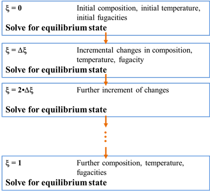
The calculation procedure for tracing a titration path is straightforward. We begin by calculating the equilibrium state of the initial system. We then incrementally change the system's bulk composition as a function of reaction progress. After each increment, we recalculate the equilibrium state.
In this lesson, we'll look at how we can use React to model reaction processes. We'll consider how species and minerals can serve to buffer the chemistry of natural systems. We start by looking at how dissolved carbonate affects how readily a solution can be acidified.
Task 1: Buffers in solution
Starting with an alkaline NaCl solution, simulate the effects of adding 0.3 moles of hydrochloric acid. Double-click on file “buffers.rea”, and when React opens, look at the Basis pane
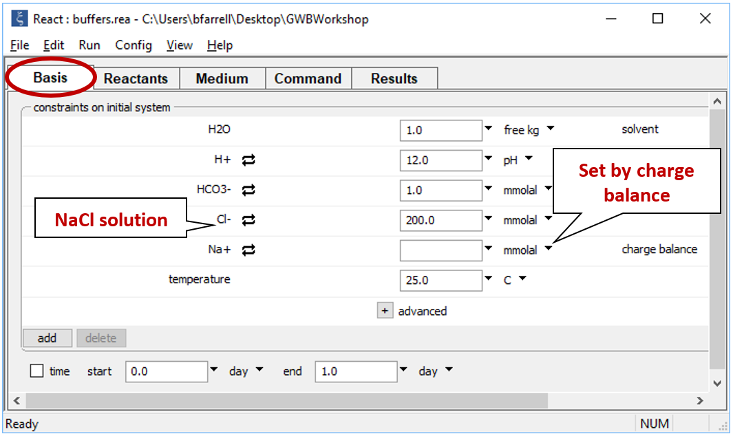
The Basis pane contains the unreacted water, a dominantly NaCl water at pH 12.
Move to the Reactants pane
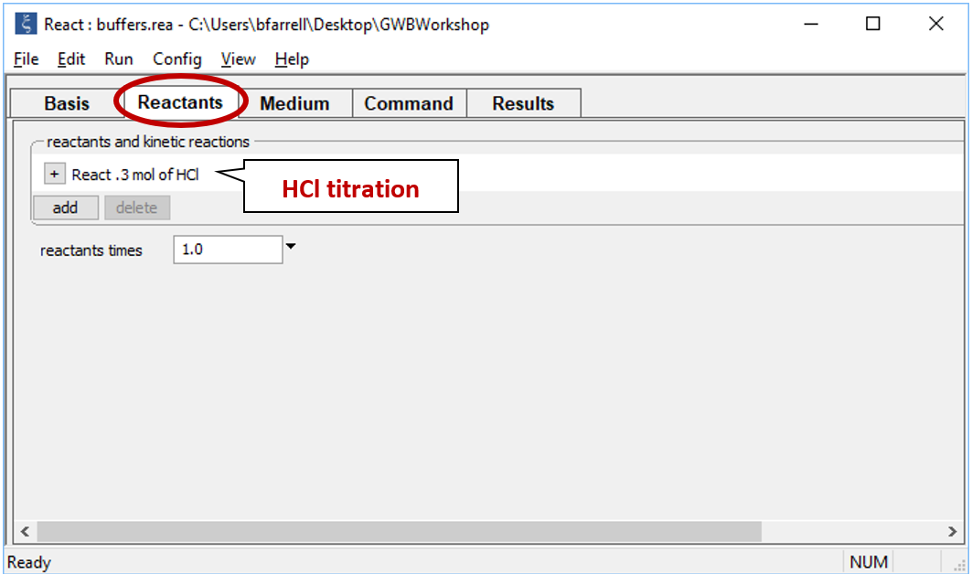
Here we've defined a reaction path in which we'll titrate 300 mmol of HCl into the initial fluid.
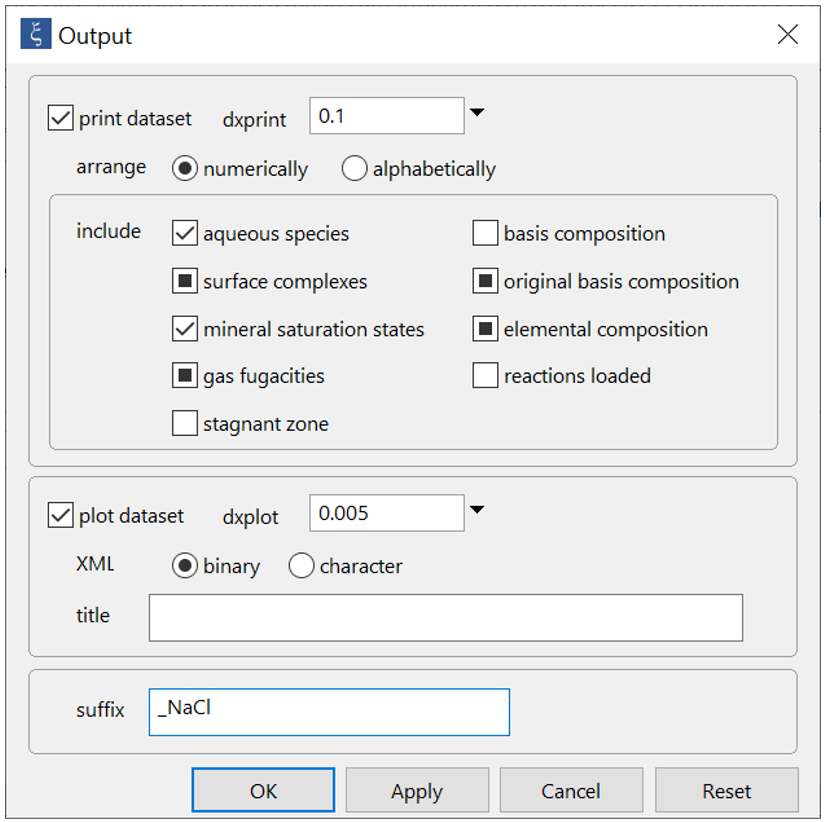
On Config → Output… set a suffix “_NaCl”
Click OK, then on the main window select Run → Go (CTRL+G). React will move to the Results pane and trace the simulation
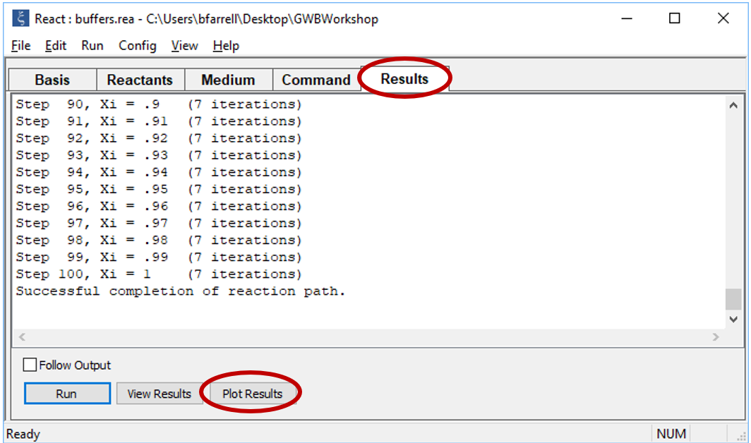
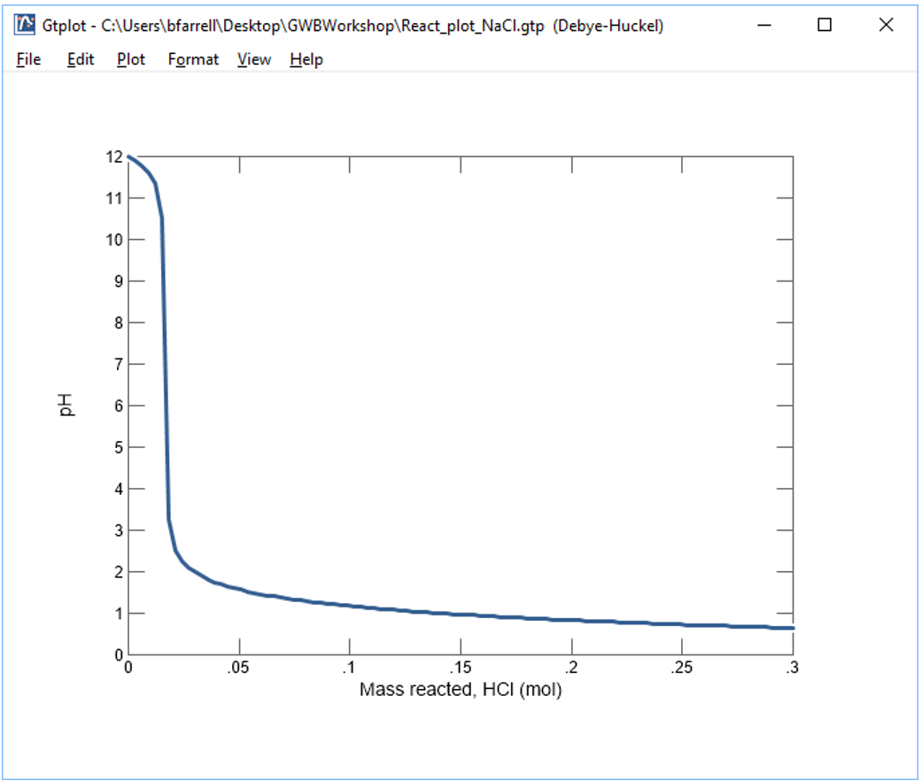
Click on the Plot Results button to launch Gtplot.
To make a plot of pH vs. the amount of HCl added to solution, configure the plot as indicated:
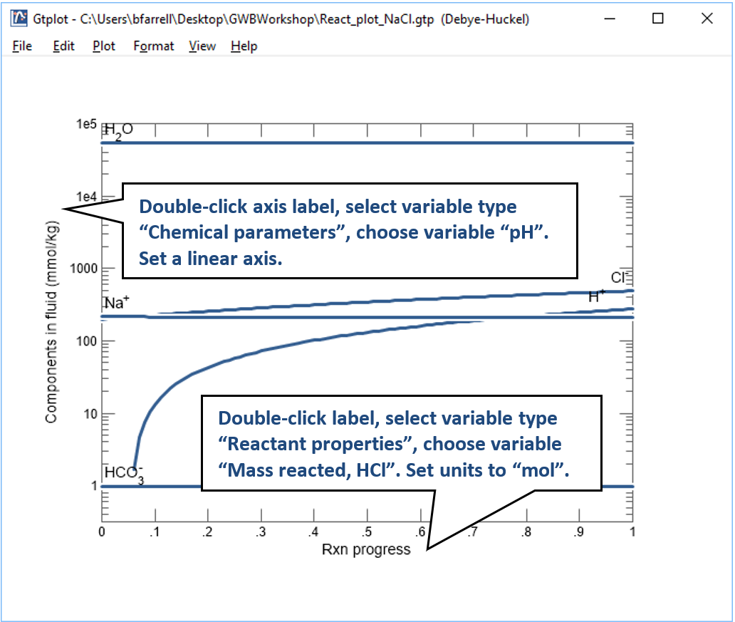
Your diagram should look like this:
Continuing in React, reverse the anion concentrations so that the fluid is dominantly an Na2CO3 solution. Set the concentration of the “HCO3-” component to “100”, and that of “Cl-” to “1”
On Config → Output… set a suffix “_Na2CO3” and rerun the simulation. Again, plot pH vs. HCl reacted.
Why do the curves for the NaCl and Na2CO3 solutions differ? How did the pH of each water change as acid was added?
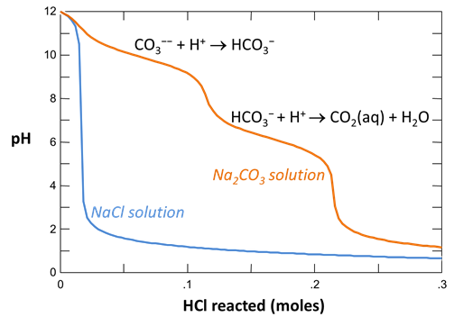
The NaCl solution is quickly driven acidic. The only buffer is the presence of OH- ions, which are quickly consumed by reaction with H+ to produce water.
The Na2CO3 solution, on the other hand, resists acidification until more than 200 mmol of HCl have been added. The two plateaus represent the buffering reactions between CO32- and HCO3-, and between HCO3- and CO2(aq). When all the CO32- and HCO3- species have been consumed, the solution quickly becomes acidic.
Plot the distribution of carbonate species in the second water vs. the amount of acid added. Choose a linear scale for the species distribution. Compare this plot to the plot above. Considering the slopes of the lines in this plot, what reactions occur among the species?
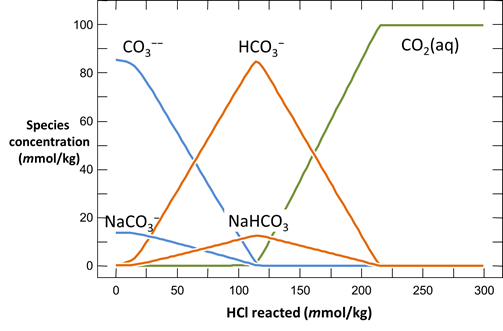
The slopes of the lines in the plot give the reaction coefficients for each species and mineral in the overall reaction. Species with negative slopes appear to the left of the reaction (with their coefficients set positive), and those with positive slopes are placed to the right. The reactant plotted on the horizontal axis appears to the left of the reaction with a coefficient of 1. In the first stage, the overall reaction is

The reaction for the second stage is

It is common practice when writing overall reactions to omit mention of ion pairs whenever they are not considered important to the point being addressed. Grouping the ion pairs with the free ions,
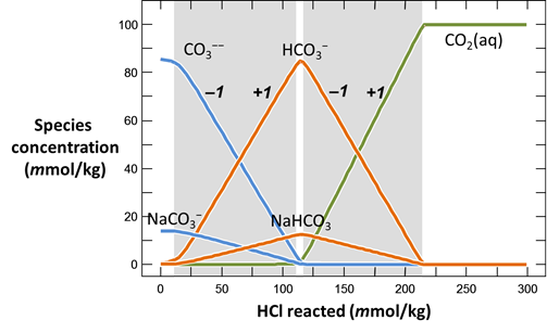
we could well write the reactions above as

and

The simplified form is not as exact but is less cluttered than the full form and shows more clearly the nature of the buffering reaction.
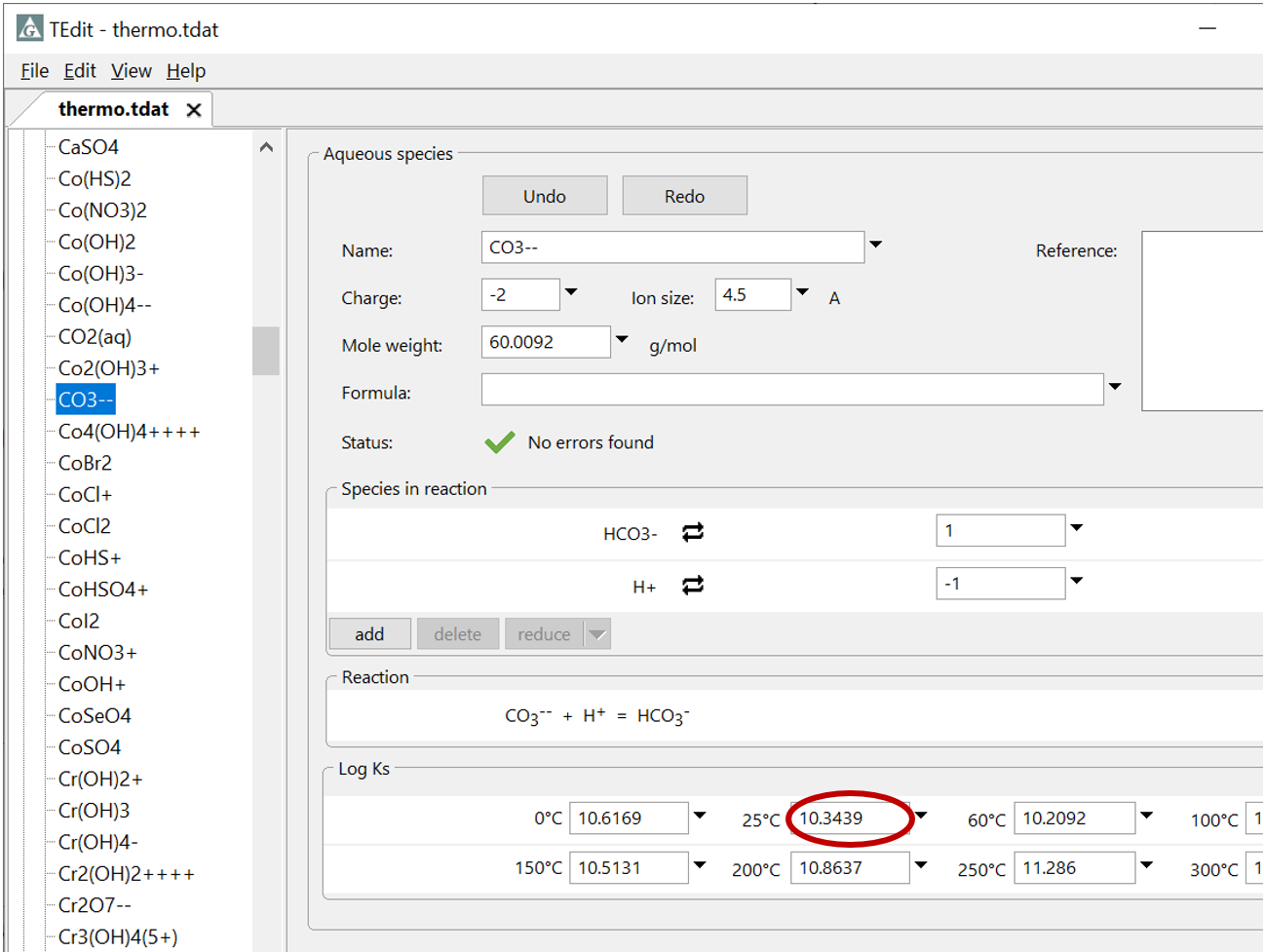
Plot the molalities of carbonate species (on a linear scale) in the second water against pH. Over which pH range does each buffering reaction proceed? Open the “thermo.tdat” database by selecting File → View. Do the theoretical crossover pHs for the buffering reactions in “thermo.tdat” agree exactly with your results? If not, why not?
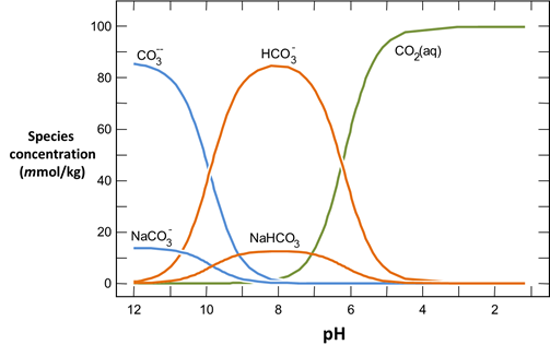
Based on the data in the thermo dataset, we would expect the crossover point for the reaction between CO32- and HCO3- to occur at pH 10.3439. This is true when we plot species' activities, but not their concentrations, as above
Task 2: Coexisting minerals as buffers
Now let's consider how minerals coexisting with the fluid might buffer pH and oxygen activity. We simulate the effects at 100°C of oxygen infiltrating a formation containing the iron mineral pyrite (FeS2) and a small amount of hematite (Fe2O3).
Double-click on file “mineral_buffers.rea”, and when React opens, look at the Basis pane
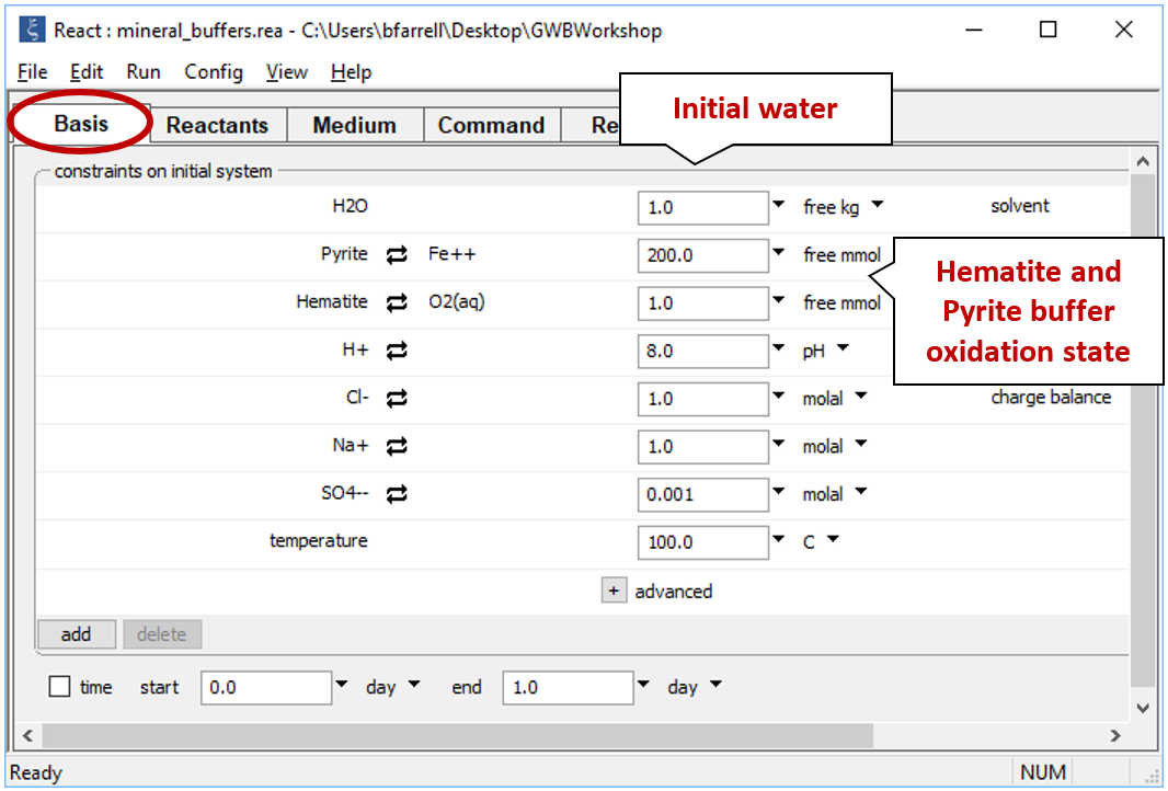
The Basis pane describes the reducing water, at equilibrium with hematite and pyrite.
Move to the Reactants pane
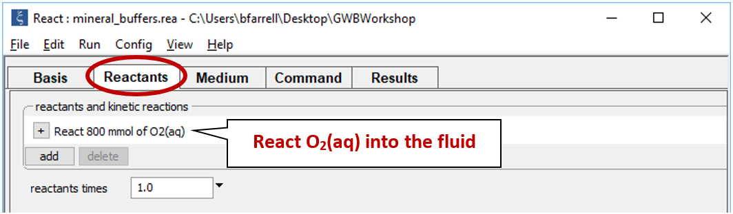
Here we've defined a reaction path in which we'll titrate 800 mmol of O2(aq) into the initial fluid.
On Config → Output… set a suffix “_mineral_buffer”
Click OK, then on the main window select Run → Go. React will move to the Results pane and trace the simulation.
Use Gtplot to render the results. From the slopes of the lines on the plots of mineral mass and species concentration versus O2(aq) reacted, determine the overall reaction occurring in the system.
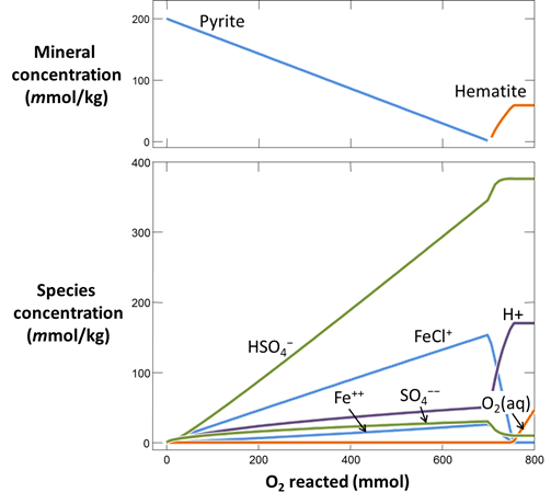
Clearly, pyrite oxidation adds iron and sulfur to the fluid. Eventually all of the pyrite dissolves and hematite begins to precipitate from the fluid, decreasing the concentration of dissolved iron.
Plot pH vs. the amount of oxygen that has diffused into the system. Why does the pH change? Also plot oxygen fugacity vs. the amount of oxygen added. The reaction between pyrite and hematite fixes the initial oxidation state. How does the oxidation state of the system change over the course of the reaction path?
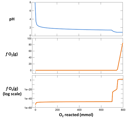
The pH changes rapidly after the initial addition of oxygen, dropping nearly six pH units, before leveling off. After about 700 mmoles of oxygen have been added to the fluid, the pH drops once again. At the same point, oxygen fugacity begins to increase after holding steady for the early portion of the reaction path.
Look at your results for this reaction path in light of a redox-pH diagram for the Fe-S-H2O system. Start Act2 by double-clicking on the script “Fe_trace.ac2”. Overlay your reaction model by dragging the “React_plot_mineral_buffers.gtp” file into the Act2 window
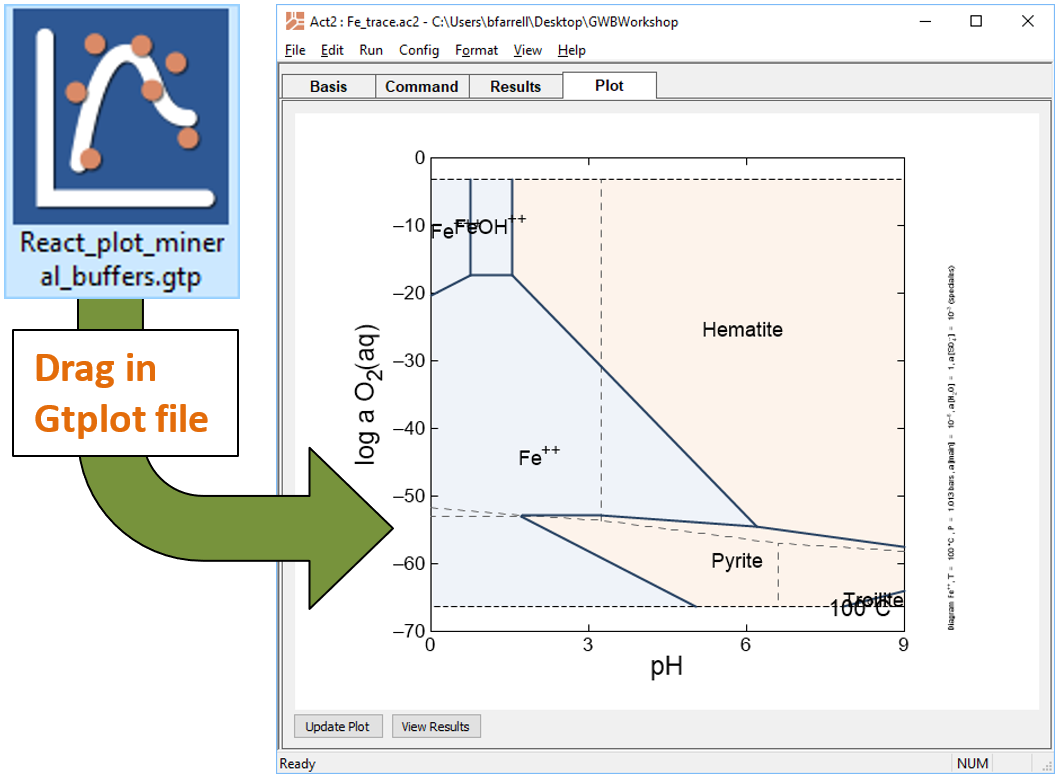
The trace command causes Act2 to project your last React run onto the diagram. From the resulting diagram, explain the main reactions that occurred in the React simulation.
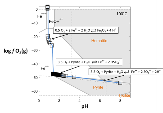
In the earliest portion of the path, the system responds to the addition of oxygen by shifting quickly toward low pH. The system's rapid acidification results from the production of H+ according to the reaction

(lumping FeCl+ together with Fe++). As the system moves to lower pH, the bisulfate species HSO4− becomes more abundant than SO4−− because of protonation of the sulfate species. At pH less than about 3, where bisulfate predominates, the dominant reaction is

Since the reaction written in terms of HSO4− produces no H+, the shift to lower pH slows and then ceases as the SO4−− in solution is depleted.
At this point, the solution remains almost fixed in oxidation state and pH, accumulating Fe++ and HSO4− as the addition of oxygen causes pyrite to dissolve. When the pyrite is exhausted, the oxygen fugacity begins to rise rapidly. As oxygen is added, it is consumed in converting the dissolved ferrous iron to hematite

which further acidifies the solution. Only when the ferrous iron is exhausted does the fluid become fully oxidized.
Task 3: Gas buffers
Now we'll investigate how gas reservoirs can buffer the chemistries of natural waters. First, we'll titrate NaOH into an acidic water that is initially in equilibrium with atmospheric CO2(g).
Double-click on file “fugacity_buffers.rea” and move to the Basis pane
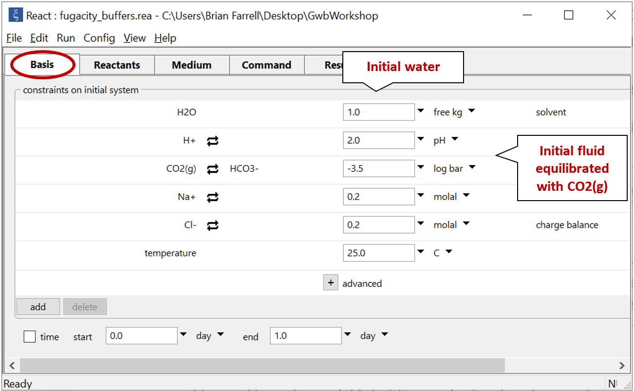
The Basis pane describes an acidic water, initially at equilibrium with atmospheric CO2(g).
Move to the Reactants pane
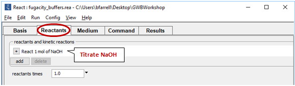
Here we've defined a reaction path in which we'll titrate NaOH into the initial fluid.
On Config → Output... set a suffix “_no_fugacity_buffer”
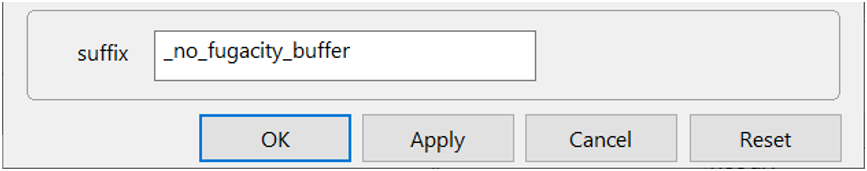
Click OK, then on the main window select Run → Go. React will move to the Results pane and trace the simulation.
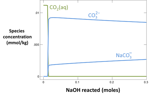
Use Gtplot to characterize the changes in pH and carbonate species' distribution accompanying the reaction. Write a balanced reaction describing the titration of NaOH into the fluid. What pH buffers were active during the reaction?
The fluid's pH quickly increases to almost 14
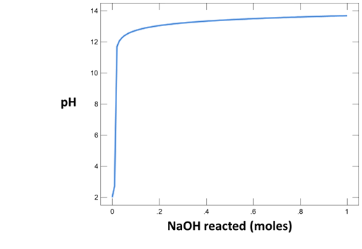
The small amount of carbon in the fluid, initially present as carbon dioxide, quickly forms carbonate
Little beyond the fluid's initial H+ content

is available to buffer pH. Once the H+ is exhausted, adding NaOH to the solution

simply produces OH−, driving the pH to high values.
Now consider the same reaction occurring in a water that remains in equilibrium with atmospheric CO2(g) over the course of the reaction.
Return to the Reactants pane and click  → Fixed → Gas... → CO2(g)
The setting fixes CO2(g) fugacity to its atmospheric value.
Set a suffix “_fix_fugacity_buffer”
and select Run → Go.
How did the presence of a CO2 buffer alter the reaction path calculated? Explain your answer, using balanced chemical reactions. Will continued addition of NaOH exhaust the CO2 buffer?
The buffered simulation, in green, is plotted together with the original calculation in blue. Where CO2 fugacity is buffered, the pH rises initially but then levels off, approaching a value of 10
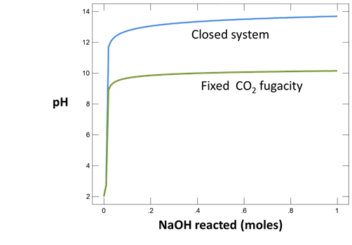
The latter path differs from the closed system calculation because of the effect of CO2(g) dissolving into the fluid. Early on, the CO2(aq) reacts to form HCO3− in response to changing pH
Since the fluid is in equilibrium with CO2(g) at a constant fugacity, however, the activity of CO2(aq) is fixed. To maintain this activity, the model transfers CO2

from gas to fluid, replacing whatever CO2(aq) has reacted to form HCO3−. The overall reaction for the earliest portion of the path is

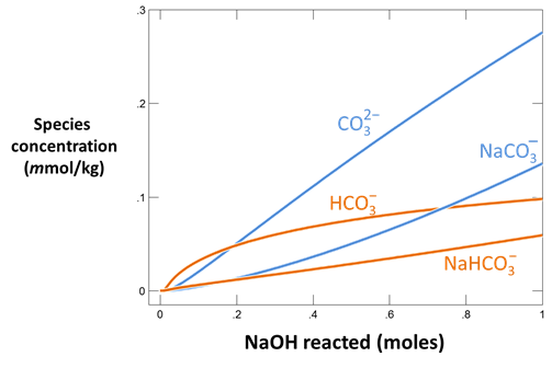
In contrast to the unbuffered case, two NaOHs are required to produce each OH− ion. As pH continues to increase, the HCO3− reacts to produce CO3−−, as shown above. At this point, a second overall reaction

becomes increasingly important. According to this reaction, adding NaOH increases the fluid's sodium and carbonate contents but does not affect the pH. The CO2, an acid gas, neutralizes the alkaline NaOH as fast as it is added. As long as CO2 is available in the gas reservoir, the fluid maintains the buffered pH.
Authors
Craig M. Bethke and Brian Farrell. © Copyright 2016–2026 Aqueous Solutions LLC. This lesson may be reproduced and modified freely to support any licensed use of The Geochemist's Workbench® software, provided that any derived materials acknowledge original authorship.
References
Bethke, C.M., 2022, Geochemical and Biogeochemical Reaction Modeling, 3rd ed. Cambridge University Press, New York, 520 pp.
Bethke, C.M., B. Farrell, and M. Sharifi, 2026, The Geochemist's Workbench®, Release 18: GWB Reaction Modeling Guide. Aqueous Solutions LLC, Champaign, IL, 219 pp.
Comfortable with buffering reactions?
Move on to the next topic, Acidity and Alkalinity, or return to the GWB Online Academy home.